More about machine learning: Machine Learning with Python
- Linear regression
- Logistic regression
- Decision trees
- Random forest
- Gradient boosting
- Machine learning with Python and Scikitlearn
- Quantile Regression
- Probabilistic Gradient Boosting (GBMLSS)
- Probabilistic Gradient Boosting (NGBoost)
- Neural Networks
- Principal Component Analysis (PCA)
- Clustering with python
- Anomaly detection with PCA
- Face Detection and Recognition
- Introduction to Graphs and Networks
Introduction
Most machine learning methods applied to regression problems model the behavior of a response variable $y$ as a function of one or more predictors $X$, and generate "point estimate" predictions. These predictions correspond to the expected value of $y$ given a specific value of the predictors ($\mathbb{E}[y|X]$).
The main limitation of these models is that they offer no information about the uncertainty associated with the predicted value. They also cannot answer questions such as:
What is the probability that, given a value of $X$, the response variable $y$ is below or above a certain threshold?
What is the probability that, given a value of $X$, the response variable $y$ falls within a given interval?
To answer these questions, probabilistic regression methods are needed — methods capable of modeling the conditional probability distribution of the response variable as a function of the predictors ($P(y|X)$).
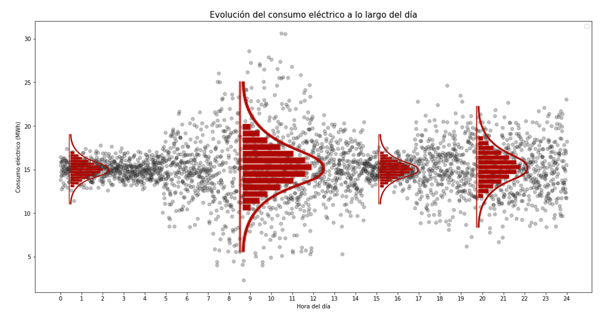
Consider the following simulated (and highly simplified) example of the evolution of electricity consumption across all households in a city as a function of the time of day.
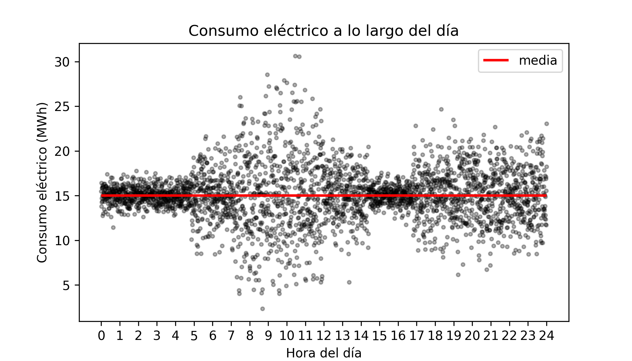
The mean electricity consumption is the same throughout the day, $\overline{consumption}$ = 15 MWh; however, its dispersion is not constant (heteroscedasticity).
Now suppose the company responsible for supplying electricity must be able to provision, at any given time, up to 50% extra electricity above average. This means a maximum of 22.5 MWh. Being prepared to supply this additional energy involves staffing and equipment costs, so the company wonders whether it is necessary to be ready to produce that amount all day, or whether it could be avoided during certain hours, thereby saving costs.
A model that only predicts the average cannot answer this question because, both at 2 a.m. and at 8 a.m., the predicted average consumption is around 15 MWh. However, the probability of reaching 22.5 MWh at 2 a.m. is practically zero, whereas it is quite plausible at 10 a.m.
One way to predict the probability that electricity consumption will exceed a given value at a given hour is to model its probability distribution as a function of the time of day.
💡 Tip
This document is part of a broader series on probabilistic machine learning.
Natural Gradient Boosting (NGBoost)
Natural Gradient Boosting (NGBoost) is a generalization of gradient boosting that is capable of estimating the parameters $\theta$ of a conditional probability distribution, thus enabling probabilistic predictions. Without going into mathematical details, the two main differences from standard gradient boosting are:
It uses natural gradient descent instead of standard gradient descent for model fitting. Unlike the standard gradient, the natural gradient corrects for the curvature of the parameter space of the distribution (using the Fisher information matrix), making the optimization steps invariant to reparameterization and improving convergence.
It estimates the parameters of a parametric probability distribution $P_{\theta}(y|X)$ instead of a point estimate $\mathbb{E}[y|X]$.
For example, if the chosen distribution is a normal, NGBoost models the mean $\mu$ and standard deviation $\sigma$ as functions of the predictors $X$. This way, it is not necessary to assume homoscedasticity (constant variance across the range of $X$).
Natural Gradient Boosting with Python
The ngboost library developed by the Stanford Machine Learning Group implements these models in Python, with an API similar to and compatible with scikit-learn.
In general terms, training an ngboost model requires defining 3 elements:
A type of base learner — by default, decision trees from scikit-learn are used.
A parametric probability distribution.
A scoring rule to guide the fitting process.
The remaining steps are identical to those in a scikit-learn gradient boosting model, including the possibility of optimizing hyperparameters via GridSearchCV and early_stopping_rounds.
The ngboost library is relatively recent and will likely continue to evolve and expand its functionality. Detailed documentation can be found in the NGBoost user guide. Currently, the available distributions and scoring rules are:
Distributions for regression
| Distribution | Parameters | Implemented Scores | Reference |
|---|---|---|---|
Normal |
loc, scale |
LogScore, CRPScore |
scipy.stats normal |
LogNormal |
s, scale |
LogScore, CRPScore |
scipy.stats lognormal |
Exponential |
scale |
LogScore, CRPScore |
scipy.stats exponential |
Distributions for classification
| Distribution | Parameters | Implemented Scores | Reference |
|---|---|---|---|
k_categorical(K) |
p0, p1... p{K-1} |
LogScore |
Categorical distribution on Wikipedia |
Bernoulli |
p |
LogScore |
Bernoulli distribution on Wikipedia |
Comparison with other probabilistic models
Given the critical need to incorporate uncertainty into decision-making, the community has developed multiple approaches to go beyond point predictions. This section compares four of the most widely used methodologies for probabilistic estimation and conditional regression.
NGBoost (Natural Gradient Boosting)
Developed by the Stanford ML Group, NGBoost is an extension of traditional Gradient Boosting aimed at uncertainty estimation.
How it works: NGBoost assumes that the target variable follows a parametric distribution $P(y|\theta)$, where $\theta$ is a parameter vector (for example, $\theta = (\mu, \sigma)$ for a Normal distribution). The model does not predict $y$ directly, but rather models the parameters $\theta$ as additive functions of the input variables $X$.
Natural Gradient: Unlike the standard gradient (used in standard gradient boosting models) which measures distances between numbers, the natural gradient measures the distance between probability distributions (using Kullback-Leibler Divergence). This makes learning more stable and mathematically elegant.
Advantage: It provides very accurate and stable uncertainty estimates.
Disadvantage: It is slower than traditional boosting models because calculating the natural gradient is computationally expensive.
BART (Bayesian Additive Regression Trees)
BART is a Bayesian model that does not rely on gradient optimization, but is instead based on Bayesian statistical sampling.
How it works: BART builds an ensemble of very simple (weak) trees. Unlike boosting, where each tree corrects the previous one, in BART the trees are modified through a process called MCMC (Markov Chain Monte Carlo). In each iteration, a modification to a tree is proposed (grow, prune, change rule, or swap) and is accepted or rejected according to the Metropolis-Hastings ratio.
Regularization (Priors): BART imposes strongly regularizing priors that penalize tree depth and leaf node weights. This forces each tree to contribute marginally (a natural shrinkage effect), preventing overfitting.
Inference Mechanism: During training, the model generates thousands of possible versions of the tree "forest." The final prediction is not a single number, but the average of all these versions. Uncertainty is obtained by observing how much the predictions vary across all generated forests.
Advantage: It does not require choosing a distribution (it is non-parametric). It is extraordinarily robust to hyperparameter tuning.
Disadvantage: The sequential MCMC process is difficult to parallelize and computationally restrictive ($O(n)$ per iteration), which limits its scalability.
GBM-LSS (Gradient Boosting for Location, Scale, and Shape)
GBM-LSS brings the concept of "Location, Scale, and Shape" to the world of high-performance Gradient Boosting (such as XGBoost or LightGBM).
How it works: It models the conditional distribution by estimating multiple parameters $\theta = (\theta_1, \theta_2, \theta_3, \theta_4)$, which typically correspond to metrics of location ($\mu$), scale ($\sigma$), skewness ($\nu$), and kurtosis ($\tau$). It allows fitting any differentiable distribution (e.g., Zero-Inflated, Tweedie, Student-t). In this sense, it is similar to NGBoost models.
Cyclic multi-parameter: The model trains trees sequentially for each parameter, meaning it assumes iterative independence between parameters.
Advantage: It is the fastest of the three and the most flexible. By leveraging infrastructures like XGBoost or LightGBM, it inherits native support for GPU parallelization, efficient early stopping, and missing value handling, allowing it to scale to millions of records.
Disadvantage: It can be difficult to configure and is sometimes unstable if the parameters are not well-balanced.
Commonly implemented through variations of algorithms such as Quantile Regression Forests (QRF) or through classic Gradient Boosting models (LightGBM, CatBoost) by changing the loss function.
Theoretical Foundation: Instead of estimating the conditional mean $\mathbb{E}[Y|X]$ or the parameters of an entire distribution $P(Y|X)$, quantile regression directly estimates a specific quantile $Q_\tau(Y|X)$ (for example, $\tau = 0.9$ for the 90th percentile). It is mathematically "distribution-free," meaning it assumes no specific shape (neither normal, gamma, nor any other).
Optimization Mechanism: It abandons mean squared error (MSE) or maximum likelihood estimation in favor of minimizing the Pinball Loss (Quantile Loss): $$L_\tau(y, \hat{y}) = \max(\tau(y - \hat{y}), (\tau - 1)(y - \hat{y}))$$ This asymmetric function penalizes underestimations and overestimations differently depending on the target quantile $\tau$.
Advantages: It is extremely robust against outliers and heteroscedasticity. It does not require prior parametric assumptions.
Limitations: While NGBoost, BART, or GBM-LSS estimate the entire probability curve (PDF), quantile regression only predicts specific predefined points (quantiles). Lacking the complete distribution, post-hoc analytical flexibility is lost: if it becomes necessary to know the exact variance or query the probability at a new threshold in the future, the model will need to be retrained to calculate those new points.
| Attribute | NGBoost | GBM-LSS | BART | Quantile Regression |
|---|---|---|---|---|
| Objective | Full Density (PDF) | Full Density (PDF) | Full Density (Posterior) | CDF Points |
| Approach | Parametric ($\mu, \sigma$) | Parametric ($\mu, \sigma, \nu, \tau$) | Bayesian (Non-parametric) | Distribution-free (Empirical) |
| Optimization | Natural Gradient (MLE/CRPS) | Taylor Expansion (Newton-Raphson) | MCMC Sampling | Pinball Loss |
| Predicted Output | Distributional parameters | Distributional parameters | Average of Markov chains | Direct intervals (e.g., $y_{10}$ to $y_{90}$) |
| Typical Issues | Slow to train | Complex to stabilize / tune | Poor scalability to Big Data | Quantile Crossing |
Example 1
An electricity supply company has hourly consumption data for all households in a city. To allocate its resources as efficiently as possible, it wants to build a probabilistic model capable of predicting, with a 90% prediction interval, the average consumption for each hour of the day. It also wants to compute the probability throughout the day that consumption exceeds a given threshold.
Libraries
The libraries used in this document are:
# Data handling
# ==============================================================================
import pandas as pd
import numpy as np
# Plotting
# ==============================================================================
import matplotlib.pyplot as plt
plt.style.use('fivethirtyeight')
plt.rcParams['lines.linewidth'] = 1.5
plt.rcParams['font.size'] = 8
# Modeling
# ==============================================================================
from ngboost import NGBRegressor
from ngboost import scores
from ngboost import distns
from sklearn.tree import DecisionTreeRegressor
from scipy import stats
# Warnings configuration
# ==============================================================================
import warnings
warnings.filterwarnings('once')
Data
Data are simulated from a normal distribution with different variance depending on the time of day.
# Simulated data
# ==============================================================================
# Simulation slightly modified from the example published in
# XGBoostLSS – An extension of XGBoost to probabilistic forecasting Alexander März
np.random.seed(seed=1234)
n = 3000
# Normal distribution with changing variance
x = np.linspace(start=0, stop= 24, num=n)
y = np.random.normal(
loc = 15,
scale = (
1 + 1.5 * ((4.8 < x) & (x < 7.2)) + 4 * ((7.2 < x) & (x < 12))
+ 1.5 * ((12 < x) & (x < 14.4)) + 2 * (x > 16.8)
)
)
Since the data were simulated using normal distributions, the theoretical quantile values are known for each hour.
# Compute the 0.1 and 0.9 quantiles for each simulated value of x
# ==============================================================================
quantile_10 = stats.norm.ppf(
q = 0.1,
loc = 15,
scale = (
1 + 1.5 * ((4.8 < x) & (x < 7.2)) + 4 * ((7.2 < x) & (x < 12))
+ 1.5 * ((12 < x) & (x < 14.4)) + 2 * (x > 16.8)
)
)
quantile_90 = stats.norm.ppf(
q = 0.9,
loc = 15,
scale = (
1 + 1.5 * ((4.8 < x) & (x < 7.2)) + 4 * ((7.2 < x) & (x < 12))
+ 1.5 * ((12 < x) & (x < 14.4)) + 2 * (x > 16.8)
)
)
# Plot
# ==============================================================================
fig, ax = plt.subplots(nrows=1, ncols=1, figsize=(7, 3.5))
ax.scatter(x, y, alpha = 0.3, c = "black", s = 8)
ax.plot(x, quantile_10, c = "black")
ax.plot(x, quantile_90, c = "black")
ax.fill_between(x, quantile_10, quantile_90, alpha=0.3, color='red',
label='Theoretical quantile interval 0.1-0.9')
ax.set_xticks(range(0, 25))
ax.set_title('Electricity consumption throughout the day')
ax.set_xlabel('Hour of the day')
ax.set_ylabel('Electricity consumption (MWh)')
plt.legend();

Model
To compute quantiles, the probabilistic distribution of the data must first be obtained. To simplify this demonstration, two assumptions are made:
It is assumed that the distribution is normal (since the data were simulated with this distribution).
Default hyperparameters are used when fitting the model.
In practice, a preliminary analysis is needed to determine both of these points (see Example 2).
# Model fitting
# ==============================================================================
model = NGBRegressor(
Dist = distns.Normal,
Base = DecisionTreeRegressor(criterion='friedman_mse', max_depth=3),
Score = scores.LogScore,
natural_gradient = True,
n_estimators = 500,
learning_rate = 0.01,
minibatch_frac = 1.0,
col_sample = 1.0,
random_state = 123,
)
model.fit(X=x.reshape(-1, 1), Y=y)
[iter 0] loss=2.5299 val_loss=0.0000 scale=2.0000 norm=4.5902 [iter 100] loss=2.2691 val_loss=0.0000 scale=2.0000 norm=4.4540 [iter 200] loss=2.2101 val_loss=0.0000 scale=1.0000 norm=2.2067 [iter 300] loss=2.1927 val_loss=0.0000 scale=2.0000 norm=4.3769 [iter 400] loss=2.1775 val_loss=0.0000 scale=2.0000 norm=4.3366
NGBRegressor(random_state=RandomState(MT19937) at 0x78D300D41140)In a Jupyter environment, please rerun this cell to show the HTML representation or trust the notebook.
On GitHub, the HTML representation is unable to render, please try loading this page with nbviewer.org.
Parameters
| Dist | <class 'ngboo...ormal.Normal'> | |
| Score | <class 'ngboo...res.LogScore'> | |
| Base | DecisionTreeR..., max_depth=3) | |
| natural_gradient | True | |
| n_estimators | 500 | |
| learning_rate | 0.01 | |
| minibatch_frac | 1.0 | |
| col_sample | 1.0 | |
| verbose | True | |
| random_state | RandomState(M...0x78D300D41140 | |
| validation_fraction | 0.1 | |
| early_stopping_rounds | None |
DecisionTreeRegressor(criterion='friedman_mse', max_depth=3)
Parameters
| criterion | 'friedman_mse' | |
| splitter | 'best' | |
| max_depth | 3 | |
| min_samples_split | 2 | |
| min_samples_leaf | 1 | |
| min_weight_fraction_leaf | 0.0 | |
| max_features | None | |
| random_state | None | |
| max_leaf_nodes | None | |
| min_impurity_decrease | 0.0 | |
| ccp_alpha | 0.0 | |
| monotonic_cst | None |
Predictions
NGBRegressor models provide two prediction methods:
predict(): returns a point estimate prediction, as most models do. This is the expected value of the response variable given the predictor values for the test observation $\mathbb{E}[y|x=x_i]$.pred_dist(): returns anngboost.distnsobject containing the conditional distribution of the response variable for the predictor values of the test observation $P(y|x=x_i)$. The estimated parameters are stored within each of these objects.
# Point estimate prediction
# ==============================================================================
point_predictions = model.predict(X=x.reshape(-1, 1))
point_predictions
array([15.02650577, 15.02650577, 15.02650577, ..., 15.13872404,
21.92369649, 17.73664598], shape=(3000,))
# Conditional distribution prediction
# ==============================================================================
dist_predictions = model.pred_dist(X=x.reshape(-1, 1))
dist_predictions
<ngboost.distns.normal.Normal at 0x78d300c58410>
# Each distns.distn object contains the estimated parameters
dist_predictions[0].params
{'loc': np.float64(15.026505766709645),
'scale': np.float64(0.9610903262391606)}
# Estimated parameters for each hour
# ==============================================================================
df_parameters = pd.DataFrame([dist.params for dist in dist_predictions])
df_parameters['hour'] = x
df_parameters
| loc | scale | hour | |
|---|---|---|---|
| 0 | 15.026506 | 0.961090 | 0.000000 |
| 1 | 15.026506 | 0.961090 | 0.008003 |
| 2 | 15.026506 | 0.961090 | 0.016005 |
| 3 | 15.026506 | 0.961090 | 0.024008 |
| 4 | 15.026506 | 0.961090 | 0.032011 |
| ... | ... | ... | ... |
| 2995 | 15.674938 | 1.789045 | 23.967989 |
| 2996 | 13.786219 | 2.108075 | 23.975992 |
| 2997 | 15.138724 | 0.974876 | 23.983995 |
| 2998 | 21.923696 | 1.180863 | 23.991997 |
| 2999 | 17.736646 | 1.102145 | 24.000000 |
3000 rows × 3 columns
Interval Predictions
Once the parameters of the conditional distribution are known, the quantiles of the expected energy consumption for each hour can be computed.
A quantile of order $\tau$ $(0 < \tau < 1)$ of a distribution is the value that marks a cut such that a proportion $\tau$ of population values is less than or equal to that value. For example, the quantile of order 0.36 leaves 36% of values below it, and the quantile of order 0.50 corresponds to 50% (the median of the distribution).
All distributions generated by NGBRegressor are scipy.stats classes, so they provide the methods pdf(), logpdf(), cdf(), ppf(), and rvs() for computing density, log-density, cumulative probability, quantiles, and sampling new values.
The steps to compute quantile intervals are:
Generate a grid of values covering the entire observed range.
For each grid value, obtain the parameters predicted by the model.
Compute quantiles of the chosen distribution using the predicted parameters.
# Compute the theoretical quantiles to define the central interval accumulating
# 90% of probability using the predicted parameters.
# ==============================================================================
grid_X = np.linspace(start=min(x), stop=max(x), num=1000)
dist_predictions = model.pred_dist(X=grid_X.reshape(-1, 1))
pred_quantile_10 = [stats.norm.ppf(q=0.1, **dist.params) for dist in dist_predictions]
pred_quantile_90 = [stats.norm.ppf(q=0.9, **dist.params) for dist in dist_predictions]
# Plot quantile interval 10%-90%
# ==============================================================================
fig, ax = plt.subplots(nrows=1, ncols=1, figsize=(7, 3.5))
ax.scatter(x, y, alpha = 0.3, c = "black", s = 8)
ax.plot(x, quantile_10, c = "black")
ax.plot(x, quantile_90, c = "black")
ax.fill_between(x, quantile_10, quantile_90, alpha=0.3, color='red',
label='Theoretical quantile interval 0.1-0.9')
ax.plot(grid_X, pred_quantile_10, c = "blue", label='Predicted quantile interval')
ax.plot(grid_X, pred_quantile_90, c = "blue")
ax.set_xticks(range(0, 25))
ax.set_title('Electricity consumption throughout the day')
ax.set_xlabel('Hour of the day')
ax.set_ylabel('Electricity consumption (MWh)')
plt.legend();

Coverage
One of the metrics used to evaluate intervals is coverage. Its value corresponds to the percentage of observations that fall within the estimated interval. Ideally, coverage should equal the confidence level of the interval, so in practice, the closer its value, the better.
In this example, quantiles 0.1 and 0.9 have been computed, so the interval has a confidence level of 80%. If the predicted interval is correct, approximately 80% of observations should fall within it.
# Interval predictions for the available observations
# ==============================================================================
dist_predictions = model.pred_dist(X=x.reshape(-1, 1))
pred_quantile_10 = [stats.norm.ppf(q=0.1, **dist.params) for dist in dist_predictions]
pred_quantile_90 = [stats.norm.ppf(q=0.9, **dist.params) for dist in dist_predictions]
# Coverage of the predicted interval
# ==============================================================================
within_interval = np.where((y >= pred_quantile_10) & (y <= pred_quantile_90), True, False)
coverage = within_interval.mean()
print(f"Coverage of the predicted interval: {100 * coverage:.2f}%")
Coverage of the predicted interval: 80.03%
Probabilistic Prediction
For example, to determine the probability that at 8 a.m. consumption exceeds 22.5 MWh, the distribution parameters are first predicted for $hour=8$ and then, using those parameters, the probability $consumption \geq 22.5$ is computed with the cumulative distribution function.
# Predict distribution parameters when hour=8
# ==============================================================================
distribution = model.pred_dist(X=np.array([8]).reshape(-1, 1))
print("Predicted distribution parameters when hour=8:")
distribution.params
Predicted distribution parameters when hour=8:
{'loc': array([14.1530422]), 'scale': array([4.52000988])}
# Probability that consumption exceeds 22.5 when hour=8
# ==============================================================================
prob_exceed = 1 - stats.norm.cdf(x=22.5, **distribution.params)[0]
print(f'P(consumption >= 22.5 MWh | hour=8) = {prob_exceed:.4f}')
P(consumption >= 22.5 MWh | hour=8) = 0.0324
According to the distribution predicted by the model, there is a 3.24% probability that consumption at 8 a.m. will be equal to or above 22.5 MWh.
If this same calculation is performed for the entire hourly range, the probability that consumption exceeds a given value throughout the day can be determined.
# Probability prediction across the full hourly range of consumption exceeding 22.5 MWh
# ==============================================================================
grid_X = np.linspace(start=0, stop=24, num=500)
dist_predictions = model.pred_dist(X=grid_X.reshape(-1, 1))
probability_predictions = [(1 - stats.norm.cdf(x=22.5, **dist.params)) for dist in dist_predictions]
fig, ax = plt.subplots(nrows=1, ncols=1, figsize=(7, 3))
ax.plot(grid_X, probability_predictions)
ax.set_xticks(range(0, 25))
ax.set_xlabel('Hour of the day')
ax.set_ylabel('P(consumption ≥ 22.5 MWh)')
ax.set_title('Probability of exceeding 22.5 MWh throughout the day');

Example 2
The dbbmi dataset (Fourth Dutch Growth Study, Fredriks et al. (2000a, 2000b)), available in the R package gamlss.data, contains information on age and body mass index (bmi) of 7,294 Dutch youths aged 0 to 20. The goal is to train a model capable of predicting quantiles of body mass index as a function of age, as this is one of the standards used to detect anomalous cases that may require medical attention.
Libraries
# Data handling
# ==============================================================================
import pandas as pd
import numpy as np
from tqdm import tqdm
# Plotting
# ==============================================================================
import matplotlib.pyplot as plt
plt.style.use('fivethirtyeight')
plt.rcParams['lines.linewidth'] = 1.5
plt.rcParams['font.size'] = 8
# Modeling
# ==============================================================================
from ngboost import NGBRegressor
from ngboost import scores
from ngboost import distns
from sklearn.tree import DecisionTreeRegressor
from sklearn.model_selection import GridSearchCV
from scipy import stats
import multiprocessing
# Warnings configuration
# ==============================================================================
import warnings
warnings.filterwarnings('once')
Data
# Load data
# ==============================================================================
url = (
'https://raw.githubusercontent.com/JoaquinAmatRodrigo/'
'Estadistica-machine-learning-python/master/data/dbbmi.csv'
)
data = pd.read_csv(url)
data.head(3)
| age | bmi | |
|---|---|---|
| 0 | 0.03 | 13.235289 |
| 1 | 0.04 | 12.438775 |
| 2 | 0.04 | 14.541775 |
# Plot distribution of bmi values
# ==============================================================================
fig, ax = plt.subplots(figsize=(6, 3))
ax.hist(data.bmi, bins=30, density=True, color='#3182bd', alpha=0.8)
ax.set_title('Distribution of body mass index values')
ax.set_xlabel('bmi')
ax.set_ylabel('density');

# Plot distribution of body mass index as a function of age
# ==============================================================================
fig, axs = plt.subplots(ncols=2, nrows=1, figsize=(8, 4), sharey=True)
data[data.age <= 2.5].plot(
x = 'age',
y = 'bmi',
c = 'black',
kind = "scatter",
alpha = 0.1,
ax = axs[0]
)
axs[0].set_ylim([10, 30])
axs[0].set_title('Age <= 2.5 years')
data[data.age > 2.5].plot(
x = 'age',
y = 'bmi',
c = 'black',
kind = "scatter",
alpha = 0.1,
ax = axs[1]
)
axs[1].set_title('Age > 2.5 years')
fig.tight_layout()
plt.subplots_adjust(top = 0.85)
fig.suptitle('Distribution of body mass index as a function of age', fontsize = 12);

This distribution exhibits three important characteristics that must be taken into account when modeling it:
The relationship between age and body mass index is neither linear nor constant. There is a notable positive relationship until about 0.25 years of age, then it stabilizes until age 10, and rises sharply again from ages 10 to 20.
Variance is heterogeneous (heteroscedasticity), being lower at younger ages and higher at older ages.
The distribution of the response variable is not normal; it shows skewness and a positive tail.
Given these characteristics, a model is needed that:
Is capable of learning non-linear relationships.
Can explicitly model variance as a function of the predictors, since it is not constant.
Is capable of learning skewed distributions with a pronounced positive tail.
Parametric Distribution Selection
NGBoost models require specifying a parametric distribution type, so the first step is to identify which of the three distributions available in NGBoost (normal, lognormal, and exponential) best fits the data.
Each distribution is fitted and evaluated graphically by overlaying it onto the histogram. Detailed information on how to compare distributions can be found in Distribution fitting and selection with Python.
def fit_plot_distribution(
x: np.ndarray,
distribution_name,
ax=None,
verbose: bool = True,
):
'''
This function overlays the density curve(s) of one or more distributions
on top of the data histogram.
Parameters
----------
x : array_like
Data used to fit the distribution.
distribution_name : str or list
Name of a distribution or list of distribution names available
in `scipy.stats`.
ax : matplotlib.axes.Axes, optional
Axes on which to draw the plot. If None, a new one is created.
verbose : bool, optional
If True, prints fitting results. For multiple distributions,
prints error warnings (default True).
Returns
-------
ax: matplotlib.axes.Axes
Generated plot
'''
# Input validation
x = np.asarray(x)
if x.size == 0:
raise ValueError("Array 'x' cannot be empty")
if not np.all(np.isfinite(x)):
raise ValueError("Array 'x' contains NaN or infinite values")
if isinstance(distribution_name, str):
distribution_name = [distribution_name]
if not isinstance(distribution_name, (list, tuple)):
raise TypeError("Parameter 'distribution_name' must be a string, list, or tuple")
# Create plot
if ax is None:
fig, ax = plt.subplots(figsize=(7,4))
# Plot histogram
ax.hist(x=x, density=True, bins=30, color="#3182bd", alpha=0.5)
ax.plot(x, np.full_like(x, -0.01), '|k', markeredgewidth=1)
ax.set_title('Distribution fit' if len(distribution_name) == 1 else
'Distribution fits')
ax.set_xlabel('x')
ax.set_ylabel('Probability density')
for name in tqdm(distribution_name):
if not hasattr(stats, name):
if verbose:
print(f"⚠️ Distribution '{name}' does not exist in scipy.stats")
continue
try:
distribution = getattr(stats, name)
parameters = distribution.fit(data=x)
is_continuous = isinstance(distribution, stats.rv_continuous)
pdf_func = distribution.pdf if is_continuous else distribution.pmf
x_hat = np.linspace(min(x), max(x), num=100)
y_hat = pdf_func(x_hat, *parameters)
ax.plot(x_hat, y_hat, linewidth=2, label=distribution.name)
except Exception as e:
if verbose:
print(f"⚠️ Error fitting distribution '{name}': {type(e).__name__}: {e}")
ax.legend(loc='best')
return ax
fig, ax = plt.subplots(figsize=(6, 3))
fit_plot_distribution(
x=data.bmi.to_numpy(),
distribution_name=['lognorm', 'norm', 'expon'],
ax=ax
);

The graphical representation provides clear evidence that, among the available distributions, the lognormal is the best fit.
Model
Unlike the previous example, cross-validation is used here to identify the optimal hyperparameters.
X = data.age.to_numpy()
y = data.bmi.to_numpy()
# Hyperparameter grid
# ==============================================================================
b1 = DecisionTreeRegressor(criterion='friedman_mse', max_depth=2)
b2 = DecisionTreeRegressor(criterion='friedman_mse', max_depth=4)
param_grid = {
'Base': [b1, b2],
'n_estimators': [100, 500, 1000]
}
# Cross-validation search
# ==============================================================================
grid = GridSearchCV(
estimator = NGBRegressor(
Dist = distns.LogNormal,
Score = scores.LogScore,
verbose = False
),
param_grid = param_grid,
scoring = 'neg_root_mean_squared_error', # Evaluates point prediction (expected value). To evaluate full distributional quality, neg-log-likelihood or CRPS would be used.
n_jobs = multiprocessing.cpu_count() - 1,
cv = 5,
verbose = 0
)
# Assign result to _ to suppress printed output
_ = grid.fit(X = X.reshape(-1, 1), y = y)
# Grid results
# ==============================================================================
results = pd.DataFrame(grid.cv_results_)
results.filter(regex = '(param.*|mean_t|std_t)')\
.drop(columns = 'params')\
.sort_values('mean_test_score', ascending = False)
| param_Base | param_n_estimators | mean_test_score | std_test_score | |
|---|---|---|---|---|
| 1 | DecisionTreeRegressor(criterion='friedman_mse'... | 500 | -2.254565 | 0.420097 |
| 2 | DecisionTreeRegressor(criterion='friedman_mse'... | 1000 | -2.256332 | 0.360156 |
| 4 | DecisionTreeRegressor(criterion='friedman_mse'... | 500 | -2.291792 | 0.307326 |
| 3 | DecisionTreeRegressor(criterion='friedman_mse'... | 100 | -2.334395 | 0.438422 |
| 5 | DecisionTreeRegressor(criterion='friedman_mse'... | 1000 | -2.372743 | 0.200955 |
| 0 | DecisionTreeRegressor(criterion='friedman_mse'... | 100 | -2.444140 | 0.651819 |
# Best hyperparameters
# ==============================================================================
print("-----------------------------------")
print("Best hyperparameters found")
print("-----------------------------------")
print(grid.best_params_, ":", grid.best_score_, grid.scoring)
-----------------------------------
Best hyperparameters found
-----------------------------------
{'Base': DecisionTreeRegressor(criterion='friedman_mse', max_depth=2), 'n_estimators': 500} : -2.2545651891289116 neg_root_mean_squared_error
# Best model found
# ==============================================================================
model = grid.best_estimator_
Interval Predictions
Once the parameters of the conditional distribution are known, the expected body mass index quantiles for each age can be computed.
# Compute the quantiles to define the central interval accumulating
# 90% of probability using the predicted parameters.
# ==============================================================================
grid_X = np.linspace(start=min(data.age), stop=max(data.age), num=2000)
dist_predictions = model.pred_dist(X=grid_X.reshape(-1, 1))
pred_quantile_10 = [stats.lognorm.ppf(q=0.1, **dist.params) for dist in dist_predictions]
pred_quantile_90 = [stats.lognorm.ppf(q=0.9, **dist.params) for dist in dist_predictions]
df_intervals = pd.DataFrame({
'age': grid_X,
'pred_quantile_10': pred_quantile_10,
'pred_quantile_90': pred_quantile_90
})
# Plot quantile interval 10%-90%
# ==============================================================================
fig, axs = plt.subplots(ncols=2, nrows=1, figsize=(10, 4.5), sharey=True)
data[data.age <= 2.5].plot(
x = 'age',
y = 'bmi',
c = 'black',
kind = "scatter",
alpha = 0.1,
ax = axs[0]
)
df_intervals[df_intervals.age <= 2.5].plot(
x = 'age',
y = 'pred_quantile_10',
c = 'red',
kind = "line",
ax = axs[0]
)
df_intervals[df_intervals.age <= 2.5].plot(
x = 'age',
y = 'pred_quantile_90',
c = 'red',
kind = "line",
ax = axs[0]
)
axs[0].set_ylim([10, 30])
axs[0].set_title('Age <= 2.5 years')
data[data.age > 2.5].plot(
x = 'age',
y = 'bmi',
c = 'black',
kind = "scatter",
alpha = 0.1,
ax = axs[1]
)
df_intervals[df_intervals.age > 2.5].plot(
x = 'age',
y = 'pred_quantile_10',
c = 'red',
kind = "line",
ax = axs[1]
)
df_intervals[df_intervals.age > 2.5].plot(
x = 'age',
y = 'pred_quantile_90',
c = 'red',
kind = "line",
ax = axs[1]
)
axs[1].set_title('Age > 2.5 years')
axs[1].get_legend().remove()
fig.tight_layout()
plt.subplots_adjust(top = 0.85)
fig.suptitle('Distribution of body mass index as a function of age', fontsize = 14);

Coverage
One of the metrics used to evaluate intervals is coverage. Its value corresponds to the percentage of observations that fall within the estimated interval. Ideally, coverage should equal the confidence level of the interval, so in practice, the closer its value, the better.
In this example, quantiles 0.1 and 0.9 were computed using a LogNormal distribution, so the interval has a confidence level of 80%. If the model and chosen distribution are correct, approximately 80% of observations should fall within it.
# Interval predictions for the available observations
# ==============================================================================
dist_predictions = model.pred_dist(X=X.reshape(-1, 1))
pred_quantile_10 = [stats.lognorm.ppf(q=0.1, **dist.params) for dist in dist_predictions]
pred_quantile_90 = [stats.lognorm.ppf(q=0.9, **dist.params) for dist in dist_predictions]
# Coverage of the predicted interval
# ==============================================================================
within_interval = np.where((y >= pred_quantile_10) & (y <= pred_quantile_90), True, False)
coverage = within_interval.mean()
print(f"Coverage of the predicted interval: {100 * coverage:.2f}%")
Coverage of the predicted interval: 82.11%
Anomalies (Outliers)
Knowing the probability distribution is useful for detecting anomalies — observations with values that are very unlikely according to the model.
For a given age, low body mass index values are indicative of potential malnutrition issues, and very high values are indicative of potential overweight problems. Using the trained model, individuals with bmi values that are highly improbable given their age are identified.
# 98% interval predictions for the available observations
# ==============================================================================
X = data.age.to_numpy()
y = data.bmi.to_numpy()
dist_predictions = model.pred_dist(X=X.reshape(-1, 1))
pred_quantile_01 = [stats.lognorm.ppf(q=0.01, **dist.params) for dist in dist_predictions]
pred_quantile_99 = [stats.lognorm.ppf(q=0.99, **dist.params) for dist in dist_predictions]
within_interval = np.where((y >= pred_quantile_01) & (y <= pred_quantile_99), True, False)
df_intervals = pd.DataFrame({
'age': X,
'bmi': y,
'pred_quantile_01': pred_quantile_01,
'pred_quantile_99': pred_quantile_99,
'within_interval': within_interval
})
df_intervals.head()
| age | bmi | pred_quantile_01 | pred_quantile_99 | within_interval | |
|---|---|---|---|---|---|
| 0 | 0.03 | 13.235289 | 11.016612 | 17.542151 | True |
| 1 | 0.04 | 12.438775 | 11.016612 | 17.542151 | True |
| 2 | 0.04 | 14.541775 | 11.016612 | 17.542151 | True |
| 3 | 0.04 | 11.773954 | 11.016612 | 17.542151 | True |
| 4 | 0.04 | 15.325614 | 11.016612 | 17.542151 | True |
Individuals for whom the model assigns a probability of occurrence equal to or below 1% are highlighted in red.
# Anomaly plot
# ==============================================================================
fig, axs = plt.subplots(ncols=2, nrows=1, figsize=(10, 4.5), sharey=True)
df_intervals[df_intervals.age <= 2.5].plot(
x = 'age',
y = 'bmi',
c = 'black',
kind = "scatter",
alpha = 0.1,
ax = axs[0]
)
df_intervals[(df_intervals.age <= 2.5) & (df_intervals.within_interval == False)].plot(
x = 'age',
y = 'bmi',
c = 'red',
kind = "scatter",
label = 'anomaly',
ax = axs[0]
)
axs[0].set_ylim([10, 30])
axs[0].set_title('Age <= 2.5 years')
df_intervals[df_intervals.age > 2.5].plot(
x = 'age',
y = 'bmi',
c = 'black',
kind = "scatter",
alpha = 0.1,
ax = axs[1]
)
df_intervals[(df_intervals.age > 2.5) & (df_intervals.within_interval == False)].plot(
x = 'age',
y = 'bmi',
c = 'red',
kind = "scatter",
ax = axs[1]
)
axs[1].set_title('Age > 2.5 years')
fig.tight_layout()
plt.subplots_adjust(top = 0.85)
fig.suptitle('Distribution of body mass index as a function of age', fontsize = 14);

Session Information
import session_info
session_info.show(html=False)
----- matplotlib 3.10.8 ngboost 0.5.10 numpy 2.1.3 pandas 2.3.3 scipy 1.15.3 session_info v1.0.1 sklearn 1.7.2 tqdm 4.67.3 ----- IPython 9.10.0 jupyter_client 8.8.0 jupyter_core 5.9.1 ----- Python 3.13.11 | packaged by Anaconda, Inc. | (main, Dec 10 2025, 21:28:48) [GCC 14.3.0] Linux-6.17.0-20-generic-x86_64-with-glibc2.39 ----- Session information updated at 2026-04-13 22:47
Citation Instructions
How to cite this document?
If you use this document or any part of it, we appreciate you citing it. Thank you!
Probabilistic gradient boosting with Python: NGBoost by Joaquín Amat Rodrigo, available under an Attribution-NonCommercial-ShareAlike 4.0 International (CC BY-NC-SA 4.0 DEED) license at https://www.cienciadedatos.net/documentos/py26-probabilistic-gradient-boosting-python-ngboost.html\n"
Did you enjoy the article? Your support matters
Your contribution helps me continue producing free educational content. Thank you so much! 😊


This document created by Joaquín Amat Rodrigo is licensed under Attribution-NonCommercial-ShareAlike 4.0 International.
You are free to:
-
Share: copy and redistribute the material in any medium or format.
-
Adapt: remix, transform, and build upon the material.
Under the following terms:
-
Attribution: You must give appropriate credit, provide a link to the license, and indicate if changes were made. You may do so in any reasonable manner, but not in any way that suggests the licensor endorses you or your use.
-
NonCommercial: You may not use the material for commercial purposes.
-
ShareAlike: If you remix, transform, or build upon the material, you must distribute your contributions under the same license as the original.