More about machine learning: Machine Learning with Python
- Linear regression
- Logistic regression
- Decision trees
- Random forest
- Gradient boosting
- Machine learning with Python and Scikitlearn
- Quantile Regression
- Probabilistic Gradient Boosting (GBMLSS)
- Probabilistic Gradient Boosting (NGBoost)
- Neural Networks
- Principal Component Analysis (PCA)
- Clustering with python
- Anomaly detection with PCA
- Face Detection and Recognition
- Introduction to Graphs and Networks

Introduction 
Most supervised machine learning models applied to regression problems generate a point estimate of the target variable $y$ given a set of predictors $\mathbf{X}$. This estimate typically corresponds to the conditional mean $\mathbb{E}[y \mid \mathbf{X}]$. While perfectly adequate for many tasks, point predictions carry a fundamental limitation: they say nothing about the uncertainty surrounding the predicted value.
Consider a company that manages electricity distribution. The grid must be provisioned to handle peak demand, not just average demand. Knowing that the expected consumption at 10 AM is 15 MWh is useful, but knowing that there is a 5% probability that it exceeds 22.5 MWh is far more actionable for capacity planning. A standard regression model cannot answer the second question.
More formally, point-estimate models do not provide:
- Prediction intervals: a range $[L, U]$ that covers the true value with a given probability, e.g., $P(L \leq y \leq U \mid \mathbf{X}) = 0.90$.
- Probability predictions: $P(y > c \mid \mathbf{X})$ for an arbitrary threshold $c$.
- Full conditional distribution $p(y \mid \mathbf{X})$, which contains all information about the response variable.
Distributional regression addresses these limitations by modelling the full conditional distribution of $y$ rather than just its mean. The output of the model is no longer a single number, but the parameters of a parametric probability distribution, for example, the mean $\mu$ and standard deviation $\sigma$ of a Normal distribution, both of which can vary as functions of $\mathbf{X}$.
Gradient Boosting Machines for Location, Scale and Shape (GBM-LSS), extend the gradient boosting framework to distributional regression. Instead of fitting a single boosting model to the conditional mean, GBM-LSS fits one gradient boosting model per distributional parameter, guiding each one towards the maximum likelihood estimate of the full distribution. The result is a flexible, non-parametric model for the entire conditional distribution $p(y \mid \mathbf{X})$.
This approach inherits all the strengths of modern gradient boosting, handling of non-linear relationships, robustness to outliers (with appropriate distributions), compatibility with heterogeneous tabular data, built-in variable selection via shrinkage, while extending its predictions from a single number to a full probability distribution.
This article covers the conceptual foundations, a comparison with alternative probabilistic approaches, the practical Python API, and two worked examples: one on simulated data with known ground truth, and one on a real-world pediatric growth dataset.
💡 Tip
This document is part of a broader series on probabilistic machine learning.
Distributional gradient boosting: GBM-LSS
Standard gradient boosting for regression trains a single ensemble of trees that maps features $\mathbf{X}$ to a prediction of the conditional mean $\mathbb{E}[y \mid \mathbf{X}]$. This is fundamentally a point prediction: one number per observation.
GBM-LSS extends this idea so that the output of the model is not one number but an entire probability distribution. To do this, it relies on the concept of distributional regression: rather than modelling only the expected value of $y$, it models all parameters of a chosen parametric distribution as functions of the predictors. For a Normal distribution, that means modelling both the mean $\mu(\mathbf{X})$ and the standard deviation $\sigma(\mathbf{X})$. For a Gamma distribution, it means modelling the shape and rate parameters. Each of those parameters gets its own gradient boosting ensemble, trained jointly to maximise the likelihood of the observed data.
The name Location, Scale and Shape comes from the generic labelling convention used in the GAMLSS framework (Rigby & Stasinopoulos, 2005), which this approach directly extends to gradient boosting trees. Location refers to where the distribution is centred ($\mu$), scale to how spread out it is ($\sigma$), and shape to asymmetry and tail behaviour ($\nu$, $\tau$). Not every distribution requires all four, a Normal distribution needs only location and scale, but the framework supports up to four independently modelled parameters. The practical consequence is that the model can capture heteroscedasticity (variance that changes with the predictors), variable skewness, and variable tail weight, none of which standard GBM can represent.
The two Python implementations covered in this article are XGBoostLSS and LightGBMLSS, both written and maintained by Alexander März. They wrap XGBoost and LightGBM respectively, extending them with distributional regression while keeping the same familiar training API.
How GBM-LSS works
Location, Scale and Shape parameters
Any continuous parametric distribution can be characterised by its parameters. The GBM-LSS framework uses the generic notation $(\mu, \sigma, \nu, \tau)$ for up to four parameters, which loosely map to:
| Parameter | Role | Example |
|---|---|---|
| $\mu$ (Location) | Where the distribution is centred | Mean of Normal, median of Laplace |
| $\sigma$ (Scale) | How spread out the distribution is | Std. dev. of Normal, scale of Gamma |
| $\nu$ (Shape 1) | Asymmetry / skewness | Degrees of freedom of Student-t |
| $\tau$ (Shape 2) | Tail weight / kurtosis | Second shape parameter in four-parameter distributions |
Not all distributions require all four parameters. A Normal distribution needs only $(\mu, \sigma)$; a Student-t needs $(\mu, \sigma, \nu)$; most four-parameter distributions are rarely needed in practice. In standard regression, only $\mu$ is modelled as a function of $\mathbf{X}$, and all other parameters are estimated as global constants. GBM-LSS models all distributional parameters as functions of $\mathbf{X}$:
$$\hat{\theta}_k(\mathbf{X}) = h_k^{-1}(F_k(\mathbf{X}))$$where $h_k$ is a link function that maps the unconstrained output of the boosting model to the valid range of parameter $k$, and $F_k$ is a gradient boosting ensemble.
The training objective: negative log-likelihood
In standard gradient boosting for regression, the model minimises the expected squared error or MAE loss. In GBM-LSS, the loss is the negative log-likelihood of the assumed distribution:
$$\mathcal{L}(\mathbf{F}) = -\sum_{i=1}^{n} \log p\!\left(y_i \mid \boldsymbol{\theta}(\mathbf{X}_i)\right)$$where $\mathbf{F} = (F_1, \ldots, F_K)$ is the vector of GBM models, one per distributional parameter, and $K$ is the number of parameters in the chosen distribution. Minimising this loss is equivalent to maximum likelihood estimation of all distributional parameters simultaneously.
Gradient boosting is applied to this objective: at each iteration $t$, a new tree is added to the model for each parameter $k$ by fitting the negative gradient (and Hessian) of $\mathcal{L}$ with respect to the current prediction:
$$r_{i,k}^{(t)} = -\left[\frac{\partial \log p(y_i \mid \boldsymbol{\theta})}{\partial F_k(\mathbf{X}_i)}\right]_{F_k = F_k^{(t-1)}}$$To compute these derivatives efficiently, frameworks like lightgbmlss leverage PyTorch's automatic differentiation capabilities. This means gradients and Hessians are estimated simultaneously for all parameters under the hood, allowing users to easily implement custom distributions without manually deriving complex analytical derivatives.
The result is $K$ gradient boosting ensembles trained jointly, each responsible for predicting one distributional parameter as a non-linear function of the predictors.
An alternative loss function supported by the library is the Continuous Ranked Probability Score (CRPS) (loss_fn="crps"). CRPS is a proper scoring rule that generalises MAE to probabilistic forecasts and has the same units as $y$. Unlike NLL, CRPS does not require specifying a distributional family — it evaluates forecast quality by comparing the predicted CDF $F$ to the observed outcome $y$:
In practice loss_fn="nll" (the default) is the most common choice; loss_fn="crps" can be useful when robustness to distributional misspecification is a priority.
Training algorithm
The GBM-LSS training algorithm proceeds as follows:
Initialise each parameter model $F_k^{(0)}$ with the MLE estimate of $\theta_k$ on the training set (a single constant per parameter that maximises the unconditional likelihood).
For each boosting iteration $t = 1, \ldots, T$:
- Compute the negative gradient (pseudo-residuals) for each parameter $k$.
- Fit a new regression tree $h_k^{(t)}$ to the pseudo-residuals for parameter $k$.
- Update $F_k^{(t)} = F_k^{(t-1)} + \eta \cdot h_k^{(t)}$, where $\eta$ is the learning rate.
- Apply the link function to map the raw prediction to the valid parameter space.
Return the final ensemble $\mathbf{F} = (F_1, \ldots, F_K)$.
After training, a prediction for a new observation $\mathbf{X}^*$ is the personalised distribution:
$$\hat{\boldsymbol{\theta}}(\mathbf{X}^*) = \left(h_1^{-1}(F_1(\mathbf{X}^*)),\ \ldots,\ h_K^{-1}(F_K(\mathbf{X}^*))\right)$$Each observation receives its own distribution $p(y \mid \hat{\boldsymbol{\theta}}(\mathbf{X}^*))$ rather than a single point estimate.
Link functions
Link functions ensure that the raw unconstrained GBM output is mapped to a value in the valid domain of each distributional parameter:
| Parameter domain | Link function | Inverse link | Typical use |
|---|---|---|---|
| $\mathbb{R}$ (unbounded) | Identity: $g(\theta) = \theta$ | $\theta = F$ | Mean of Normal or Laplace |
| $(0, \infty)$ (strictly positive) | Log: $g(\theta) = \log(\theta)$ | $\theta = e^F$ | Scale parameters, Gamma shape |
| $(0, 1)$ (probability) | Logit: $g(\theta) = \log\frac{\theta}{1-\theta}$ | $\theta = \sigma(F)$ | Zero-inflation probability |
For example, when fitting a Normal distribution, the mean $\mu$ uses the identity link (any real number is valid), and the standard deviation $\sigma$ uses the log link (it must be strictly positive). The library handles link function application automatically — the user only needs to choose the distribution family.
Available distributions
One of the most consequential modelling decisions is the choice of distributional family. GBM-LSS supports a wide range of parametric distributions. Below is a practical guide organised by the type of response variable.
Continuous symmetric distributions
| Distribution | Parameters | Use case |
|---|---|---|
| Normal | $\mu \in \mathbb{R}$, $\sigma > 0$ | Continuous data, roughly symmetric errors; baseline choice |
| Student-t | $\mu \in \mathbb{R}$, $\sigma > 0$, $\nu > 0$ | Heavy-tailed data, robust to outliers; generalises Normal |
| Laplace | $\mu \in \mathbb{R}$, $\sigma > 0$ | Heavier tails than Normal (exponential decay), sharp peak at mode; analogous to L1 loss |
| Logistic | $\mu \in \mathbb{R}$, $\sigma > 0$ | Slightly heavier tails than Normal |
The Student-t distribution is particularly valuable in practice. When the degrees-of-freedom parameter $\nu$ is large, it approximates a Normal distribution; as $\nu$ decreases, the tails become heavier. This provides robustness to outliers without requiring the analyst to pre-specify outlier thresholds.
Continuous asymmetric distributions (positive domain)
| Distribution | Parameters | Use case |
|---|---|---|
| LogNormal | $\mu \in \mathbb{R}$, $\sigma > 0$ | Positive data with right skew; income, prices |
| Gamma | $\mu > 0$, $\sigma > 0$ | Positive data; insurance claims, waiting times |
| Beta | $\mu \in (0,1)$, $\sigma > 0$ | Proportions and rates bounded in $(0, 1)$ |
| Weibull | $\mu > 0$, $\sigma > 0$ | Failure and survival times |
| Gumbel | $\mu \in \mathbb{R}$, $\sigma > 0$ | Extreme values, return levels |
Discrete and count data
| Distribution | Parameters | Use case |
|---|---|---|
| Poisson | $\mu > 0$ | Count data; assumes mean = variance |
| Negative Binomial | $\mu > 0$, $\sigma > 0$ | Overdispersed count data (variance > mean) |
| Zero-Inflated Poisson (ZIP) | $\mu > 0$, $\pi \in (0,1)$ | Counts with excess zeros |
| Zero-Inflated Negative Binomial (ZINB) | $\mu > 0$, $\sigma > 0$, $\pi$ | Overdispersed counts with excess zeros |
Advanced distribution modeling (Multivariate, Mixtures, and Flows)
Beyond standard univariate distributions, the GBM-LSS framework is generic enough to handle highly complex modeling scenarios:
- Multivariate Targets: Predicting $D$-dimensional responses simultaneously (e.g., Multivariate Gaussian or Student-t) by modeling not just the means and variances, but also the covariance matrices (using, for example, Cholesky decomposition or Low-Rank approximations) as a function of the predictors.
- Mixture Distributions: Approximating multi-modal data by combining multiple component distributions (e.g., a Gaussian Mixture where the weights, means, and variances of each component depend on covariates).
- Normalizing Flows: For extremely complex, non-parametric distributions, the framework supports Normalizing Flows (like Neural Spline Flows) which apply bijective transformations to turn a simple base distribution into a realistic target distribution.
How to choose the right distribution
Domain knowledge: Start with the constraints the response variable must satisfy:
- Is $y$ strictly positive? → Gamma, LogNormal, Weibull
- Is $y$ bounded in $[0, 1]$? → Beta
- Is $y$ an integer (count)? → Poisson, Negative Binomial
- Does $y$ have a point mass at zero but is otherwise continuous? → Zero-Adjusted distributions (ZAGamma, ZALN, ZABeta)
Exploratory data analysis: Visualise the marginal distribution of $y$:
- Symmetric, bell-shaped → Normal, Student-t
- Right-skewed, strictly positive → LogNormal, Gamma
- Heavy tails on both sides → Student-t
- Sharp peak → Laplace
Automated selection (lightgbmlss): The lightgbmlss library provides a dist_select helper function (via DistributionClass) that fits each candidate distribution to the target variable by maximum likelihood and returns them ranked by negative log-likelihood (NLL). The distribution with the lowest NLL best explains the observed data. The function also plots the density of the target variable alongside the fitted densities of all candidates.
Residual diagnostics: After fitting a candidate model, inspect the PIT (Probability Integral Transform) histogram, the distribution of $F(y_i \mid \hat{\boldsymbol{\theta}}_i)$ across the test set. A well-calibrated model produces a flat histogram; deviations indicate mis-specification:
- U-shaped → tails too light (model is over-confident)
- Hump-shaped → tails too heavy (model is under-confident)
- Skewed → asymmetry of the distribution is mis-specified
GBM-LSS vs other probabilistic approaches
Several approaches to distributional or probabilistic regression are available in Python. Understanding their trade-offs upfront helps motivate the choice of GBM-LSS.
GBM-LSS vs Quantile Regression
| Aspect | Quantile Regression | GBM-LSS |
|---|---|---|
| Output | Specific quantiles | Full parametric distribution |
| Distributional assumption | None (non-parametric) | Parametric (distribution must be chosen) |
| $P(y > c \mid \mathbf{X})$ for arbitrary $c$ | Requires interpolation | Exact, from the CDF |
| Quantile crossing | Possible | Impossible (parametric coherence) |
| Number of models trained | One per quantile | One per distributional parameter |
| Captures heteroscedasticity | Yes | Yes |
| Captures variable skewness | Partially | Yes |
Choose Quantile Regression when no parametric distribution is a reasonable assumption (e.g., multimodal or mixture-shaped responses), or when only a fixed set of quantile levels is needed.
Choose GBM-LSS when a parametric family is plausible, you want a fully coherent distributional description that supports computing any quantile, any tail probability, and any moment, without training separate models.
GBM-LSS vs NGBoost
| Aspect | NGBoost | GBM-LSS |
|---|---|---|
| Optimisation | Natural gradient (Fisher information scaled) | Standard gradient (NLL loss) |
| GBDT backend | Custom (ngboost library) | XGBoost / LightGBM (optimised) |
| Speed | Slower | Faster (especially on large datasets) |
| Distributional families | Limited (~5) | Extensive (30+) |
| Feature importance | Standard per-tree importance | SHAP per distributional parameter |
| Active development | Slower (as of 2026) | Active |
In practice, GBM-LSS outperforms NGBoost on large tabular datasets in both speed and distributional accuracy, due to the highly optimised XGBoost and LightGBM backends. NGBoost's natural gradient update can be advantageous when the likelihood surface is poorly conditioned, but this is rarely decisive in practice.
Summary recommendation
| Situation | Recommended approach |
|---|---|
| Quick baseline, only a few quantile levels needed | Quantile regression (GBM with pinball loss) |
| Small dataset, statistical inference with coefficients | GAMLSS (R) or NGBoost |
| Large tabular dataset, known parametric family | GBM-LSS (XGBoostLSS / LightGBMLSS) |
| Unknown or complex distributional shape | Quantile regression or normalising flows |
| Full Bayesian inference required | PyMC or Stan |
Example 1: Simulated heteroscedastic data
The first example uses simulated data where the variance of the response variable changes as a function of the predictor. This is a canonical case where standard regression fails and distributional modelling shines.
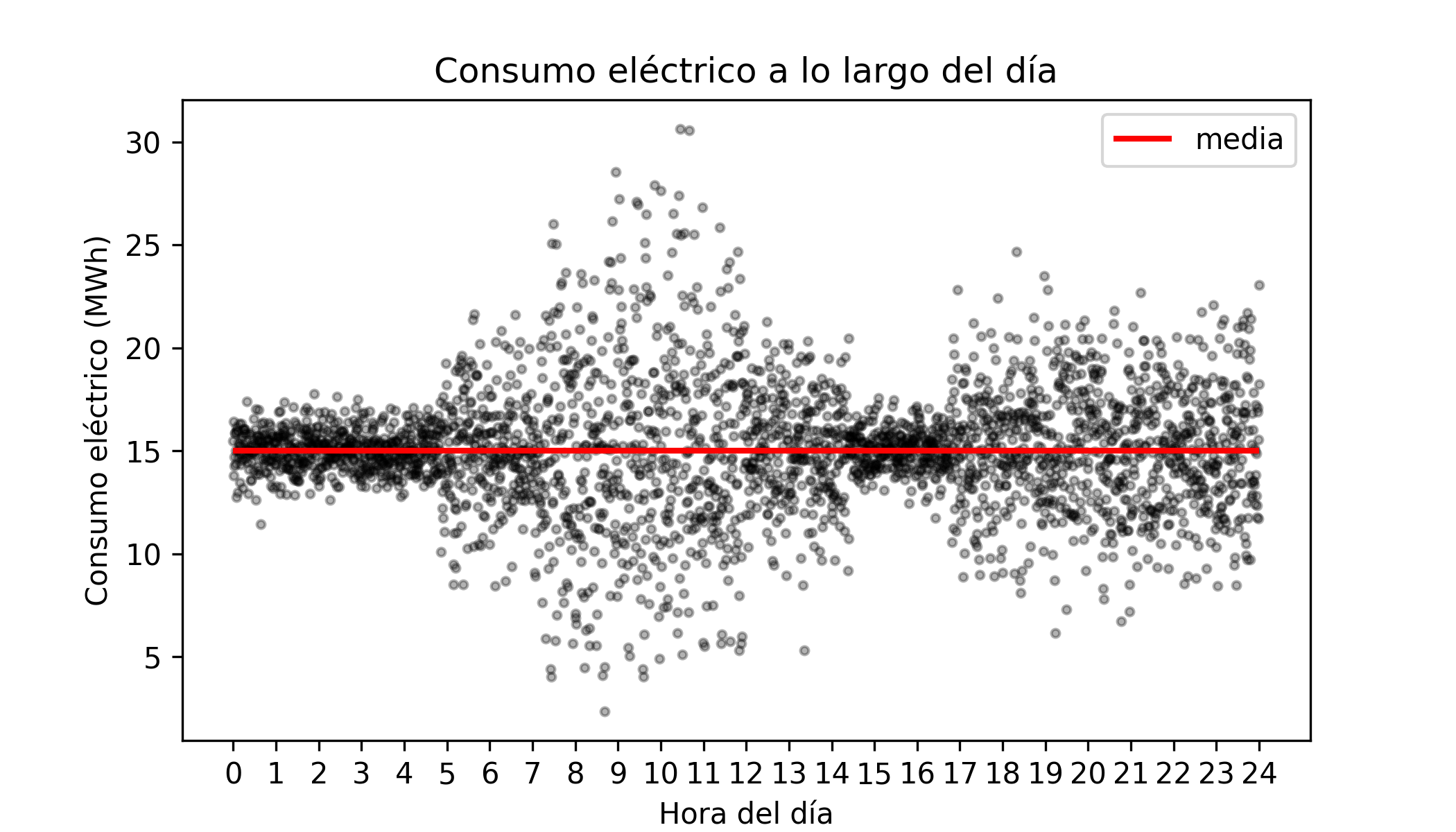
Problem setting: A utility company monitors hourly electricity consumption across thousands of households. The average consumption is roughly constant throughout the day (~15 MWh), but the variability is not: consumption is tightly clustered at night and highly dispersed during peak morning and evening hours. The company wants to:
- Predict the full distribution of consumption for each hour.
- Compute prediction intervals with 90% coverage.
- Estimate the probability that consumption exceeds a threshold at each hour.
Libraries and data
# Libraries
# ==============================================================================
import numpy as np
import pandas as pd
import matplotlib.pyplot as plt
import lightgbm as lgb
from lightgbmlss.model import LightGBMLSS
from lightgbmlss.distributions.Gaussian import Gaussian
import lightgbmlss.distributions.Gaussian as Gaussian_mod
import lightgbmlss.distributions.StudentT as StudentT_mod
import lightgbmlss.distributions.Gamma as Gamma_mod
import lightgbmlss.distributions.LogNormal as LogNormal_mod
from sklearn.model_selection import train_test_split
from scipy import stats
import warnings
warnings.filterwarnings('once')
plt.style.use('fivethirtyeight')
plt.rcParams['lines.linewidth'] = 1.5
plt.rcParams['font.size'] = 8
✏️ Note
Users can switch from the LightGBM-based model to the XGBoost-based model simply by replacing lightgbmlss with xgboostlss.
# Simulated data
# ==============================================================================
# Simulation slightly modified from the example published in
# XGBoostLSS - An extension of XGBoost to probabilistic forecasting Alexander März
np.random.seed(1234)
n = 3000
X = np.linspace(0, 24, n)
y = np.random.normal(
loc=15,
scale=(
1
+ 1.5 * ((4.8 < X) & (X < 7.2))
+ 4.0 * ((7.2 < X) & (X < 12.0))
+ 1.5 * ((12.0 < X) & (X < 14.4))
+ 2.0 * (X > 16.8)
)
)
The data is generated from $\mathcal{N}(15, \sigma^2(t))$ where $\sigma(t)$ changes with the hour of the day. Standard GBM captures the constant mean well but cannot represent the changing variance.
# Compute the 0.1 and 0.9 quantiles for each simulated value of X
# ==============================================================================
quantile_10 = stats.norm.ppf(
q = 0.1,
loc = 15,
scale = (
1 + 1.5 * ((4.8 < X) & (X < 7.2)) + 4 * ((7.2 < X) & (X < 12))
+ 1.5 * ((12 < X) & (X < 14.4)) + 2 * (X > 16.8)
)
)
quantile_90 = stats.norm.ppf(
q = 0.9,
loc = 15,
scale = (
1 + 1.5 * ((4.8 < X) & (X < 7.2)) + 4 * ((7.2 < X) & (X < 12))
+ 1.5 * ((12 < X) & (X < 14.4)) + 2 * (X > 16.8)
)
)
# Plot
# ==============================================================================
fig, ax = plt.subplots(figsize=(7, 3.5))
ax.scatter(X, y, alpha = 0.3, c = "black", s = 8)
ax.hlines(y=15, xmin=0, xmax=24, colors='tomato', lw=2, label='True mean (15 MWh)')
ax.plot(X, quantile_10, c = "black")
ax.plot(X, quantile_90, c = "black")
ax.fill_between(
X, quantile_10, quantile_90, alpha=0.3, color='red',
label='Theoretical quantile interval 0.1-0.9'
)
ax.set_xlabel('Hour of day')
ax.set_ylabel('Consumption (MWh)')
ax.set_title('Hourly electricity consumption')
ax.set_xticks(range(0, 25, 2))
ax.legend()
plt.tight_layout()

Model training
# Train-test split
# ==============================================================================
X_train, X_test, y_train, y_test = train_test_split(
X.reshape(-1, 1), y, test_size=0.2, random_state=42, shuffle=True
)
# When using XGBoostLSS data must be transformed into a xgb.DMatrix
# dX_train = xgb.DMatrix(X_train, label=y_train)
# dX_test = xgb.DMatrix(X_test, label=y_test)
# When using LightGBMLSS data must be transformed into a lgb.Dataset
dX_train = lgb.Dataset(X_train, label=y_train)
dX_test = lgb.Dataset(X_test, label=y_test)
print(f"Train set: {X_train.shape[0]} samples")
print(f"Test set: {X_test.shape[0]} samples")
Train set: 2400 samples Test set: 600 samples
When fitting the GBM-LSS model, it is required to specify a distributional family. Each distribution class accepts three key arguments:
- stabilization : "None" | "MAD" | "L2" — gradient/Hessian stabilization method
- response_fn : "exp" | "softplus" — inverse link for positive parameters (e.g. scale)
- loss_fn : "nll" | "crps" — training loss (negative log-likelihood or CRPS)
In this case, we choose the Normal distribution, which has two parameters: $\mu$ (mean) and $\sigma$ (standard deviation). The mean is modelled with the identity link, and the standard deviation with the log link to ensure positivity. The training objective is the negative log-likelihood of the Normal distribution.
# Model specification
# ==============================================================================
model = LightGBMLSS(
Gaussian(stabilization="None", response_fn="exp", loss_fn="nll")
)
To find the optimal hyperparameters, a Bayesian search is performed using the integration with Optuna provided by the library. The search optimises the validation negative log-likelihood over a predefined hyperparameter space, using early stopping to prevent overfitting. The best model is then refit on the entire training set with the optimal hyperparameters.
# Hyperparameter optimization
# ==============================================================================
# !pip install optuna-integration[lightgbm]
params_dict = {
"learning_rate": ["float", {"low": 1e-5, "high": 1, "log": True}],
"max_depth": ["int", {"low": 1, "high": 10, "log": False}],
"min_gain_to_split": ["float", {"low": 1e-8, "high": 40, "log": False}],
"min_sum_hessian_in_leaf": ["float", {"low": 1e-8, "high": 500, "log": True}],
"subsample": ["float", {"low": 0.2, "high": 1.0, "log": False}],
"feature_fraction": ["float", {"low": 0.2, "high": 1.0, "log": False}],
"boosting": ["categorical", ["gbdt"]],
}
opt_params = model.hyper_opt(
hp_dict = params_dict,
train_set = dX_train,
num_boost_round=100, # Number of boosting iterations.
nfold=5, # Number of cv-folds.
early_stopping_rounds=20, # Number of early-stopping rounds
max_minutes=10, # Time budget in minutes, i.e., stop study after the given number of minutes.
n_trials=30, # The number of trials. If this argument is set to None, there is no limitation on the number of trials.
silence=True, # Controls the verbosity of the trail, i.e., user can silence the outputs of the trail.
seed=123, # Seed used to generate cv-folds.
hp_seed=6715 # Seed for random number generator used in the Bayesian hyperparameter search.
)
0%| | 0/30 [00:00<?, ?it/s]
Hyper-Parameter Optimization successfully finished.
Number of finished trials: 30
Best trial:
Value: 2.265606331242457
Params:
learning_rate: 0.9273640481563128
max_depth: 1
min_gain_to_split: 0.035986405436204016
min_sum_hessian_in_leaf: 0.025909830444300425
subsample: 0.7788823527111574
feature_fraction: 0.6019028154022705
boosting: gbdt
opt_rounds: 31
The model is trained with the best hyperparameters found in the search.
# Train model with optimal hyperparameters
# ==============================================================================
n_rounds = opt_params.pop("opt_rounds")
model.train(
params = opt_params,
train_set = dX_train,
num_boost_round = n_rounds
)
Predictions
lightgbmlss provides three different options for making predictions:
samples: draws $n$ samples from the predicted distribution.quantiles: calculates quantiles from the predicted distribution.parameters: returns predicted distributional parameters.
When using prediction type samples, the output is a DataFrame with one row per observation in the test set and n_samples columns, each containing a draw from the predicted distribution for that observation. These represent possible future outcomes consistent with the model's uncertainty.
# Sample from predicted distribution
# ==============================================================================
sample_predictions = model.predict(data=X_test, pred_type="samples", n_samples=50)
sample_predictions
| y_sample0 | y_sample1 | y_sample2 | y_sample3 | y_sample4 | y_sample5 | y_sample6 | y_sample7 | y_sample8 | y_sample9 | ... | y_sample40 | y_sample41 | y_sample42 | y_sample43 | y_sample44 | y_sample45 | y_sample46 | y_sample47 | y_sample48 | y_sample49 | |
|---|---|---|---|---|---|---|---|---|---|---|---|---|---|---|---|---|---|---|---|---|---|
| 0 | 15.697314 | 16.262325 | 16.202932 | 15.307989 | 17.619083 | 13.853810 | 15.308901 | 12.309548 | 15.882831 | 19.780371 | ... | 17.041090 | 16.348074 | 14.840222 | 11.370354 | 12.450369 | 13.575173 | 13.577733 | 16.836323 | 13.708682 | 18.007421 |
| 1 | 14.166789 | 18.025551 | 23.503204 | 19.067127 | 11.026548 | 14.392353 | 7.978942 | 4.036101 | 25.193146 | 14.973810 | ... | 11.270795 | 14.132236 | 15.480999 | 10.183868 | 19.415047 | 27.263340 | 12.544895 | 14.446023 | 19.760115 | 10.920843 |
| 2 | 14.586010 | 13.869585 | 15.001597 | 16.088562 | 14.989753 | 15.055332 | 13.881459 | 14.251566 | 15.061149 | 15.794733 | ... | 15.848513 | 15.297975 | 16.091333 | 14.388843 | 15.170838 | 14.735168 | 14.798789 | 13.742496 | 13.630329 | 13.089798 |
| 3 | 14.592566 | 14.624412 | 14.269474 | 15.491898 | 15.569511 | 16.288342 | 15.164846 | 14.566668 | 13.327274 | 14.233431 | ... | 13.844853 | 15.285441 | 14.233530 | 14.675815 | 15.908656 | 15.858871 | 15.202689 | 15.007872 | 14.247766 | 14.850210 |
| 4 | 16.392326 | 14.859611 | 19.943062 | 13.869667 | 17.015881 | 15.606420 | 22.863440 | 16.727417 | 20.740311 | 12.586379 | ... | 16.827066 | 13.654144 | 14.565105 | 19.044834 | 13.281296 | 10.824958 | 10.942783 | 11.074723 | 12.510992 | 13.662723 |
| ... | ... | ... | ... | ... | ... | ... | ... | ... | ... | ... | ... | ... | ... | ... | ... | ... | ... | ... | ... | ... | ... |
| 595 | 14.199569 | 12.481850 | 15.573352 | 15.122883 | 15.642666 | 13.908475 | 16.400906 | 15.557431 | 17.194227 | 17.689520 | ... | 15.000471 | 17.024361 | 14.361902 | 15.227952 | 14.057050 | 16.765730 | 15.868464 | 15.708106 | 14.718128 | 13.703343 |
| 596 | 16.862871 | 15.523841 | 14.538917 | 13.587122 | 15.685340 | 16.660721 | 15.864644 | 14.723064 | 15.661668 | 17.678423 | ... | 14.425453 | 14.341781 | 15.765164 | 14.548565 | 13.399756 | 17.723585 | 16.486721 | 17.126137 | 14.486805 | 17.241503 |
| 597 | 16.452101 | 14.660017 | 14.022560 | 14.965786 | 15.117435 | 14.897168 | 15.493895 | 15.492521 | 15.704017 | 15.135339 | ... | 14.843552 | 14.960234 | 15.990202 | 14.974794 | 15.501653 | 16.243484 | 15.444390 | 14.754246 | 14.522926 | 15.973195 |
| 598 | 14.150993 | 16.409111 | 15.669437 | 15.129354 | 20.987328 | 15.376616 | 15.166396 | 15.373619 | 15.436773 | 14.702501 | ... | 14.456417 | 17.717783 | 14.643255 | 11.609344 | 17.478497 | 14.445816 | 14.792369 | 15.499956 | 14.302234 | 15.070537 |
| 599 | 18.794319 | 22.029449 | 16.802168 | 12.680256 | 8.722343 | 13.182603 | 15.911584 | 6.012594 | 20.524622 | 18.866379 | ... | 15.987385 | 6.264203 | 9.161081 | 5.458413 | 18.129385 | 17.038593 | 17.099699 | 26.817642 | 18.101303 | 17.728611 |
600 rows × 50 columns
# Prediction of quantiles
# ==============================================================================
quantile_predictions = model.predict(data=X_test, pred_type="quantiles", quantiles=[0.1, 0.9])
quantile_predictions
| quant_0.1 | quant_0.9 | |
|---|---|---|
| 0 | 12.138686 | 17.828659 |
| 1 | 8.832257 | 21.029195 |
| 2 | 13.532447 | 16.402666 |
| 3 | 13.928053 | 16.376365 |
| 4 | 11.775336 | 19.083310 |
| ... | ... | ... |
| 595 | 13.756510 | 16.352524 |
| 596 | 13.673839 | 16.496371 |
| 597 | 13.872277 | 16.089009 |
| 598 | 12.043160 | 18.024937 |
| 599 | 9.239491 | 21.524747 |
600 rows × 2 columns
# Prediction of distributional parameters
# ==============================================================================
parameter_predictions = model.predict(data=X_test, pred_type="parameters")
parameter_predictions
| loc | scale | |
|---|---|---|
| 0 | 14.931164 | 2.270949 |
| 1 | 15.008944 | 4.737135 |
| 2 | 14.931164 | 1.137141 |
| 3 | 15.172076 | 0.985543 |
| 4 | 15.406059 | 2.829181 |
| ... | ... | ... |
| 595 | 15.053152 | 0.985543 |
| 596 | 15.050743 | 1.137141 |
| 597 | 15.008944 | 0.855896 |
| 598 | 14.931164 | 2.270949 |
| 599 | 15.332772 | 4.737135 |
600 rows × 2 columns
# Plot quantile interval 10%-90%
# ==============================================================================
sort_idx = np.argsort(X_test.ravel())
X_test_sorted = X_test.ravel()[sort_idx]
quantile_predictions_sorted = quantile_predictions.iloc[sort_idx]
fig, ax = plt.subplots(nrows=1, ncols=1, figsize=(7, 3.5))
ax.scatter(X, y, alpha = 0.3, c = "black", s = 8)
ax.plot(X, quantile_10, c = "black")
ax.plot(X, quantile_90, c = "black")
ax.fill_between(X, quantile_10, quantile_90, alpha=0.3, color='red',
label='Theoretical quantile interval 0.1-0.9')
ax.plot(X_test_sorted, quantile_predictions_sorted.iloc[:, 0], c = "blue", label='Predicted quantile interval')
ax.plot(X_test_sorted, quantile_predictions_sorted.iloc[:, 1], c = "blue")
ax.set_xticks(range(0, 25))
ax.set_title('Electricity consumption throughout the day')
ax.set_xlabel('Hour of the day')
ax.set_ylabel('Electricity consumption (MWh)')
plt.legend();

Coverage
One of the metrics used to evaluate intervals is coverage. Its value corresponds to the percentage of observations that fall within the estimated interval. Ideally, empirical coverage should equal the nominal coverage level of the interval. A well-calibrated model should achieve empirical coverage close to the nominal level.
In this example, quantiles 0.1 and 0.9 have been computed, so the interval has a nominal coverage level of 80%. If the predicted interval is correct, approximately 80% of observations should fall within it.
# Coverage of the predicted interval
# ==============================================================================
lower = quantile_predictions.iloc[:, 0].to_numpy()
upper = quantile_predictions.iloc[:, 1].to_numpy()
coverage = ((y_test >= lower) & (y_test <= upper)).mean()
mean_width = (upper - lower).mean()
print(f'Empirical 80% PI coverage : {coverage:.3f}')
print(f'Mean interval width : {mean_width:.3f} (MWh)')
Empirical 80% PI coverage : 0.747 Mean interval width : 6.470 (MWh)
Probabilistic Prediction
For example, to determine the probability that at 8 a.m. consumption exceeds 22.5 MWh, the distribution parameters are first predicted for $hour=8$ and then, using those parameters, the probability $consumption \geq 22.5$ is computed with the cumulative distribution function.
# Predict distribution parameters when hour=8
# ==============================================================================
x_new = np.array([[8.0]])
params_at_8 = model.predict(data=x_new, pred_type="parameters")
print("Predicted distribution parameters when hour=8:")
print(params_at_8)
Predicted distribution parameters when hour=8:
loc scale
0 15.008944 4.737135
# Probability that consumption exceeds 22.5 when hour=8
# ==============================================================================
# Column names depend on the chosen distribution (e.g., 'loc'/'scale' for Gaussian)
mu_8 = params_at_8['loc'].to_numpy()[0]
sigma_8 = params_at_8['scale'].to_numpy()[0]
prob_exceed = 1 - stats.norm.cdf(22.5, loc=mu_8, scale=sigma_8)
print(f'P(consumption >= 22.5 MWh | hour=8) = {prob_exceed:.4f}')
P(consumption >= 22.5 MWh | hour=8) = 0.0569
According to the distribution predicted by the model, there is a 5.69% probability that consumption at 8 a.m. will be equal to or above 22.5 MWh.
If this same calculation is performed for the entire hourly range, the probability that consumption exceeds a given value throughout the day can be determined.
# Probability prediction across the full hourly range of consumption exceeding 22.5 MWh
# ==============================================================================
hours = np.linspace(0, 24, 500)
d_hours = hours.reshape(-1, 1)
params_hours = model.predict(data=d_hours, pred_type="parameters")
prob_hours = 1 - stats.norm.cdf(
22.5,
loc=params_hours['loc'].to_numpy(),
scale=params_hours['scale'].to_numpy()
)
fig, ax = plt.subplots(figsize=(7, 3.5))
ax.plot(hours, prob_hours)
ax.set_xlabel('Hour of the day')
ax.set_ylabel('P(consumption ≥ 22.5 MWh)')
ax.set_title('Probability of exceeding 22.5 MWh throughout the day')
ax.set_xticks(range(0, 25, 2))
plt.tight_layout()

Example 2
The dbbmi dataset (Fourth Dutch Growth Study, Fredriks et al. (2000a, 2000b)), available in the R package gamlss.data, contains information on age and body mass index (bmi) of 7,294 Dutch youths aged 0 to 20. The goal is to train a model capable of predicting quantiles of body mass index as a function of age, as this is one of the standards used to detect anomalous cases that may require medical attention.
Libraries and data
# Libraries
# ==============================================================================
import numpy as np
import pandas as pd
import matplotlib.pyplot as plt
import lightgbm as lgb
from lightgbmlss.model import LightGBMLSS
from lightgbmlss.distributions.Gaussian import Gaussian
from lightgbmlss.distributions.Gamma import Gamma
from lightgbmlss.distributions.LogNormal import LogNormal
from lightgbmlss.distributions.StudentT import StudentT
from lightgbmlss.distributions.distribution_utils import DistributionClass
import lightgbmlss.distributions.Gaussian as Gaussian_mod
import lightgbmlss.distributions.StudentT as StudentT_mod
import lightgbmlss.distributions.Gamma as Gamma_mod
import lightgbmlss.distributions.LogNormal as LogNormal_mod
import warnings
warnings.filterwarnings('once')
plt.style.use('fivethirtyeight')
plt.rcParams['lines.linewidth'] = 1.5
plt.rcParams['font.size'] = 8
# Load data
# ==============================================================================
url = (
'https://raw.githubusercontent.com/JoaquinAmatRodrigo/'
'Estadistica-machine-learning-python/master/data/dbbmi.csv'
)
data = pd.read_csv(url)
data.head(3)
| age | bmi | |
|---|---|---|
| 0 | 0.03 | 13.235289 |
| 1 | 0.04 | 12.438775 |
| 2 | 0.04 | 14.541775 |
# Plot distribution of bmi values
# ==============================================================================
fig, ax = plt.subplots(figsize=(6, 3))
ax.hist(data.bmi, bins=30, density=True, color='#3182bd', alpha=0.8)
ax.set_title('Distribution of body mass index values')
ax.set_xlabel('bmi')
ax.set_ylabel('density');

# Plot distribution of body mass index as a function of age
# ==============================================================================
fig, axs = plt.subplots(ncols=2, nrows=1, figsize=(8, 4), sharey=True)
data[data.age <= 2.5].plot(
x = 'age',
y = 'bmi',
c = 'black',
kind = "scatter",
alpha = 0.1,
ax = axs[0]
)
axs[0].set_ylim([10, 30])
axs[0].set_title('Age <= 2.5 years')
data[data.age > 2.5].plot(
x = 'age',
y = 'bmi',
c = 'black',
kind = "scatter",
alpha = 0.1,
ax = axs[1]
)
axs[1].set_title('Age > 2.5 years')
fig.tight_layout()
plt.subplots_adjust(top = 0.85)
fig.suptitle('Distribution of body mass index as a function of age', fontsize = 12);

This distribution exhibits three important characteristics that must be taken into account when modeling it:
The relationship between age and body mass index is neither linear nor constant. There is a notable positive relationship until about 0.25 years of age, then it stabilizes until age 10, and rises sharply again from ages 10 to 20.
Variance is heterogeneous (heteroscedasticity), being lower at younger ages and higher at older ages.
The distribution of the response variable is not normal; it shows skewness and a positive tail.
Given these characteristics, a model is needed that:
Is capable of learning non-linear relationships.
Can explicitly model variance as a function of the predictors, since it is not constant.
Is capable of learning skewed distributions with a pronounced positive tail.
Distribution selection
lightgbmlss provides an automated distribution selection procedure via DistributionClass.dist_select(). The function fits each candidate distribution to the target variable by maximum likelihood and ranks them by negative log-likelihood (NLL). A lower NLL indicates a better fit to the marginal (unconditional) distribution of the response (ignoring the features $\\mathbf{X}$).
# Distribution selection
# ==============================================================================
xgblss_dist_class = DistributionClass()
candidate_distributions = [Gaussian_mod, StudentT_mod, Gamma_mod, LogNormal_mod]
dist_nll = xgblss_dist_class.dist_select(
target=data['bmi'].to_numpy(),
candidate_distributions=candidate_distributions,
max_iter=50,
plot=True,
figure_size=(6, 3)
)
dist_nll

| nll | distribution | |
|---|---|---|
| rank | ||
| 1 | 17688.355825 | LogNormal |
| 2 | 17807.554688 | Gamma |
| 3 | 18133.892757 | Gaussian |
| 4 | 18175.127931 | StudentT |
Based on the NLL ranking, we select the distribution with the lowest value and proceed with model training. For this data set, LogNormal ranks highest, which makes sense given the positive skew and heavy tail observed in the distribution of body mass index.
Model training and hyperparameter tuning
# Train-test split
# ==============================================================================
X_train, X_test, y_train, y_test = train_test_split(
data['age'].to_numpy().reshape(-1, 1),
data['bmi'].to_numpy(),
test_size=0.2,
random_state=42
)
# Model training with the selected distribution and hyperparameter optimization
# ==============================================================================
# When using XGBoostLSS data must be transformed into a xgb.DMatrix
# d_data = xgb.DMatrix(X_train, label=y_train)
# When using LightGBMLSS data must be transformed into a lgb.Dataset
d_data = lgb.Dataset(X_train, label=y_train)
model = LightGBMLSS(
LogNormal(stabilization='None', response_fn='exp', loss_fn='nll')
)
params_dict = {
"learning_rate": ["float", {"low": 1e-5, "high": 1, "log": True}],
"max_depth": ["int", {"low": 1, "high": 10, "log": False}],
"min_gain_to_split": ["float", {"low": 1e-8, "high": 40, "log": False}],
"min_sum_hessian_in_leaf": ["float", {"low": 1e-8, "high": 500, "log": True}],
"subsample": ["float", {"low": 0.2, "high": 1.0, "log": False}],
"feature_fraction": ["float", {"low": 0.2, "high": 1.0, "log": False}],
"boosting": ["categorical", ["gbdt"]],
}
opt_params = model.hyper_opt(
hp_dict=params_dict,
train_set=d_data,
num_boost_round=100,
nfold=5,
early_stopping_rounds=10,
max_minutes=10,
n_trials=30,
silence=True,
seed=123,
hp_seed=123
)
0%| | 0/30 [00:00<?, ?it/s]
Hyper-Parameter Optimization successfully finished.
Number of finished trials: 30
Best trial:
Value: 2.0346465443268174
Params:
learning_rate: 0.7526113148050829
max_depth: 1
min_gain_to_split: 0.12693190605161014
min_sum_hessian_in_leaf: 1.17102461864558e-08
subsample: 0.9928628563764392
feature_fraction: 0.20415744257468788
boosting: gbdt
opt_rounds: 100
# Train model with optimal hyperparameters
# ==============================================================================
n_rounds = opt_params.pop('opt_rounds')
model.train(opt_params, d_data, num_boost_round=n_rounds)
Predictions and prediction intervals
Once the model is trained, the goal is to predict quantiles of BMI as a function of age, not a single expected value, but the shape of the full conditional distribution $p(\text{bmi} \mid \text{age})$ at each point.
Concretely, three quantile curves are predicted over a fine grid of age values:
- q0.05 and q0.95: the lower and upper bounds of a 90% prediction interval. For any given age, 90% of children are expected to have a BMI within this range.
- q0.50: the predicted median, a robust measure of central tendency for the right-skewed BMI distribution.
A regular grid of 500 evenly-spaced age values (rather than the observed ages) is used so the resulting curves are smooth, making the heteroscedasticity and non-linearity visually clear across the full age range.
# Prediction of the median (50% quantile) and the 90% prediction interval
# ==============================================================================
age_grid = np.linspace(data['age'].min(), data['age'].max(), 500)
quantiles_to_predict = [0.05, 0.5, 0.95]
quantile_grid = model.predict(
data=age_grid.reshape(-1, 1), pred_type='quantiles', quantiles=quantiles_to_predict
)
quantile_grid.head(3)
| quant_0.05 | quant_0.5 | quant_0.95 | |
|---|---|---|---|
| 0 | 12.119442 | 13.910258 | 15.860954 |
| 1 | 12.080288 | 13.831336 | 15.894178 |
| 2 | 13.200316 | 14.995238 | 16.919324 |
# Plot
# ==============================================================================
q_grid = quantile_grid.to_numpy() # shape (500, 3): q0.05, q0.50, q0.95
mask_young_grid = age_grid <= 2.5
mask_old_grid = age_grid > 2.5
fig, axs = plt.subplots(ncols=2, nrows=1, figsize=(9, 4.5), sharey=True)
for ax, gmask, dmask, title in zip(
axs,
[mask_young_grid, mask_old_grid],
[data['age'] <= 2.5, data['age'] > 2.5],
['Age ≤ 2.5 years', 'Age > 2.5 years']
):
ax.scatter(data.loc[dmask, 'age'], data.loc[dmask, 'bmi'], c='black', alpha=0.1, s=6)
ax.fill_between(
age_grid[gmask], q_grid[gmask, 0], q_grid[gmask, 2],
alpha=0.3, color='tomato', label='90% prediction interval'
)
ax.plot(age_grid[gmask], q_grid[gmask, 1], color='tomato', lw=2, label='Median (q0.50)')
ax.plot(age_grid[gmask], q_grid[gmask, 0], color='tomato', lw=1, ls='--', label='q0.05 / q0.95')
ax.plot(age_grid[gmask], q_grid[gmask, 2], color='tomato', lw=1, ls='--')
ax.set_title(title)
ax.set_xlabel('Age (years)')
ax.set_ylabel('BMI')
axs[0].legend(fontsize=7)
fig.suptitle('Predicted quantiles of BMI by age (LogNormal GBM-LSS)', fontsize=11)
plt.tight_layout()

Finally, the empirical coverage of the 90% prediction interval is calculated on the held-out test set, where a well-calibrated model should achieve coverage close to 0.90.
# Prediction of quantiles
# ==============================================================================
quantile_predictions = model.predict(
data=X_test,
pred_type="quantiles",
quantiles=[0.05, 0.95]
)
quantile_predictions
| quant_0.05 | quant_0.95 | |
|---|---|---|
| 0 | 13.938657 | 21.610874 |
| 1 | 17.045627 | 25.072260 |
| 2 | 14.604642 | 18.645010 |
| 3 | 13.751138 | 19.467578 |
| 4 | 14.599775 | 21.713120 |
| ... | ... | ... |
| 1454 | 14.551365 | 18.590945 |
| 1455 | 16.931873 | 25.026875 |
| 1456 | 14.720979 | 19.045074 |
| 1457 | 16.014579 | 23.116499 |
| 1458 | 14.618010 | 18.566463 |
1459 rows × 2 columns
# Coverage of the predicted interval
# ==============================================================================
lower = quantile_predictions.iloc[:, 0].to_numpy()
upper = quantile_predictions.iloc[:, 1].to_numpy()
coverage = ((y_test >= lower) & (y_test <= upper)).mean()
mean_width = (upper - lower).mean()
print(f'Empirical 90% PI coverage : {coverage:.3f}')
print(f'Mean interval width : {mean_width:.3f}')
Empirical 90% PI coverage : 0.906 Mean interval width : 6.159
Citation
How to cite this document
If you use this document or any part of it, please acknowledge the source, thank you!
Probabilistic Gradient Boosting with Python: A Guide to GBM-LSS by Joaquín Amat Rodrigo available under Attribution-NonCommercial-ShareAlike 4.0 International (CC BY-NC-SA 4.0 DEED) at https://cienciadedatos.net/documentos/py26b-probabilistic-gradient-boosting-python-gbmlss.html
Did you like the article? Your support is important
Your contribution will help me to continue generating free educational content. Many thanks! 😊


This work by Joaquín Amat Rodrigo, Javier Escobar Ortiz is licensed under a Attribution-NonCommercial-ShareAlike 4.0 International.
Allowed:
-
Share: copy and redistribute the material in any medium or format.
-
Adapt: remix, transform, and build upon the material.
Under the following terms:
-
Attribution: You must give appropriate credit, provide a link to the license, and indicate if changes were made. You may do so in any reasonable manner, but not in any way that suggests the licensor endorses you or your use.
-
NonCommercial: You may not use the material for commercial purposes.
-
ShareAlike: If you remix, transform, or build upon the material, you must distribute your contributions under the same license as the original.