More about machine learning: Machine Learning with Python
- Linear regression
- Logistic regression
- Decision trees
- Random forest
- Gradient boosting
- Machine learning with Python and Scikitlearn
- Neural Networks
- Principal Component Analysis (PCA)
- Clustering with python
- Face Detection and Recognition
- Introduction to Graphs and Networks
Introduction
Decision trees are predictive models formed by binary rules (yes/no) that distribute observations based on their attributes to predict the value of the response variable.
Many predictive methods generate global models where a single equation applies to the entire sample space. When the use case involves multiple predictors interacting in complex and non-linear ways, it is very difficult to find a single global model capable of reflecting the relationship between variables. Tree-based statistical and machine learning methods encompass a set of non-parametric supervised techniques that segment the predictor space into simple regions, within which it is easier to handle interactions. This characteristic provides much of their potential.
Tree-based methods have become a benchmark in the predictive field due to the good results they generate in very diverse problems. Throughout this document, we explore how decision trees (classification and regression) are built and predicted, which are fundamental elements of more complex predictive models such as Random Forest and Gradient Boosting Machine.
Advantages
Trees are easy to interpret even when relationships between predictors are complex.
Models based on a single tree (not the case for random forest, boosting) can be graphically represented even when the number of predictors is greater than 3.
Trees can theoretically handle both numerical and categorical predictors without creating dummy variables or one-hot-encoding. In practice, this depends on the implementation of the algorithm in each library.
Being non-parametric methods, no specific distribution is required.
Generally, they require much less data cleaning and preprocessing compared to other statistical learning methods (for example, they do not require standardization).
They are not significantly influenced by outliers.
If the value of a predictor is not available for an observation, a prediction can still be obtained using all observations belonging to the last reached node, even if a terminal node cannot be reached. The prediction accuracy will be reduced, but at least it can be obtained.
They are very useful in data exploration, allowing for quick and efficient identification of the most important variables (predictors).
They are capable of automatically selecting predictors.
They can be applied to regression and classification problems.
Disadvantages
The predictive capacity of models based on a single tree is significantly lower than that achieved with other models. This is due to their tendency for overfitting and high variance. However, more complex techniques exist that, by combining multiple trees (bagging, random forest, boosting), greatly improve this problem.
They are sensitive to imbalanced training data (one class dominates over the others).
When dealing with continuous predictors, they lose some information by categorizing them at the time of node splitting.
As described later, the creation of tree branches is achieved through the recursive binary splitting algorithm. This algorithm identifies and evaluates possible splits for each predictor according to a certain measure (RSS, Gini, entropy...). Continuous predictors have a higher probability of containing, just by chance, an optimal cut point, so they tend to be favored in tree creation.
They are not capable of extrapolating outside the range of predictors observed in the training data.
Decision Trees in Python
The main implementation of decision trees in Python is available in the scikit-learn library through the DecisionTreeClassifier and DecisionTreeRegressor classes. An important feature for those who have used other implementations is that, in scikit-learn, it is necessary to convert categorical variables into dummy variables (one-hot-encoding).
Regression Trees
Regression trees are the subtype of prediction trees applied when the response variable is continuous. Generally, in training a regression tree, observations are distributed through bifurcations (nodes) generating the tree structure until a terminal node is reached. When predicting a new observation, the tree is traversed according to the value of its predictors until one of the terminal nodes is reached. The tree's prediction is the mean of the response variable of the training observations in that same terminal node.
Tree Training
The training process of a prediction tree (regression or classification) is divided into two stages:
Successive division of the predictor space generating non-overlapping regions (terminal nodes) $R_1$, $R_2$, $R_3$, ..., $R_j$. Although theoretically regions could have any shape, limiting them to rectangular regions (multi-dimensional) greatly simplifies the construction process and facilitates interpretation.
Prediction of the response variable in each region.
Despite the simplicity with which the tree construction process can be summarized, it is necessary to establish a methodology that allows creating the regions $R_1$, $R_2$, $R_3$, ..., $R_j$, or equivalently, deciding where splits are introduced: in which predictors and at what values. This is where regression and classification tree algorithms differ.
In regression trees, the criterion most frequently used to identify splits is the Residual Sum of Squares (RSS). The goal is to find the $J$ regions $(R_1$,..., $R_j)$ that minimize the total Residual Sum of Squares (RSS):
$$RSS=\displaystyle\sum_{j=1}^J \displaystyle\sum_{i \in R_j}(y_i -\hat{y}_{R_j})^2 ,$$where $\hat{y}_{R_j}$ is the mean of the response variable in region $R_j$. A less technical description is that we seek a distribution of regions such that the sum of squared deviations between observations and the mean of the region to which they belong is as small as possible.
Unfortunately, it is not possible to consider all possible partitions of the predictor space. For this reason, recursive binary splitting is used. This solution follows the same idea as stepwise (backward or forward) predictor selection in multiple linear regression; it does not evaluate all possible regions but achieves a good computation-result balance.
Recursive binary splitting
The goal of the recursive binary splitting method is to find, in each iteration, the predictor $X_j$ and the cut point (threshold) $s$ such that, if observations are distributed in the regions $\{X|X_j < s \}$ and $\{X|X_j \geq s \}$, the greatest possible reduction in RSS is achieved. The algorithm followed is:
The process starts at the top of the tree, where all observations belong to the same region.
All possible cut points $s$ are identified for each of the predictors ($X_1$, $X_2$,..., $X_p$). In the case of qualitative predictors, the possible cut points are each of their levels. For continuous predictors, their values are ordered from smallest to largest, and the midpoint between each pair of values is used as a cut point.
The total RSS achieved with each possible split identified in step 2 is calculated.
where the first term is the RSS of region 1 and the second term is the RSS of region 2, each region being the result of separating observations according to predictor $j$ and value $s$.
The predictor $X_j$ and the cut point $S$ that results in the lowest total RSS are selected, that is, resulting in the most homogeneous splits possible. If two or more splits achieve the same improvement, the choice between them is random.
Steps 1 to 4 are repeated iteratively for each of the regions created in the previous iteration until a stop rule is reached. Some of the most used are: reaching a maximum depth, no region containing less than n observations, the tree having a maximum of terminal nodes, or the addition of more nodes not reducing the error by at least a minimum %.
This methodology implies two facts:
Each optimal split is identified according to the impact it has at that moment. It is not considered if it is the split that will lead to better trees in future splits.
In each split, a single predictor is evaluated asking binary questions (yes, no), which generates two new tree branches per split. Although it is possible to evaluate more complex splits, asking a question about multiple variables at once is equivalent to asking multiple questions about individual variables.
✏️ Note
Algorithms implementing recursive binary splitting usually incorporate strategies to avoid evaluating all possible cut points. For example, for continuous predictors, a histogram grouping values is first created, and then cut points of each histogram region (bin) are evaluated.
Tree Prediction
After creating a tree, training observations are grouped in terminal nodes. To predict a new observation, the tree is traversed based on the values of its predictors until reaching one of the terminal nodes. In the case of regression, the predicted value is usually the mean of the response variable of the training observations in that same node. Although the mean is the most used value, any other can be used (median, quantile...).
Suppose we have 10 observations, each with a response variable value $Y$ and predictors $X$.
| id | 1 | 2 | 3 | 4 | 5 | 6 | 7 | 8 | 9 | 10 |
| Y | 10 | 18 | 24 | 8 | 2 | 9 | 16 | 10 | 20 | 14 |
| X | ... | ... | ... | ... | ... | ... | ... | ... | ... | ... |
The following image shows how the prediction of the tree would be for a new observation. The path to reach the final node is highlighted. In each terminal node, the index of the training observations that are part of it is detailed.
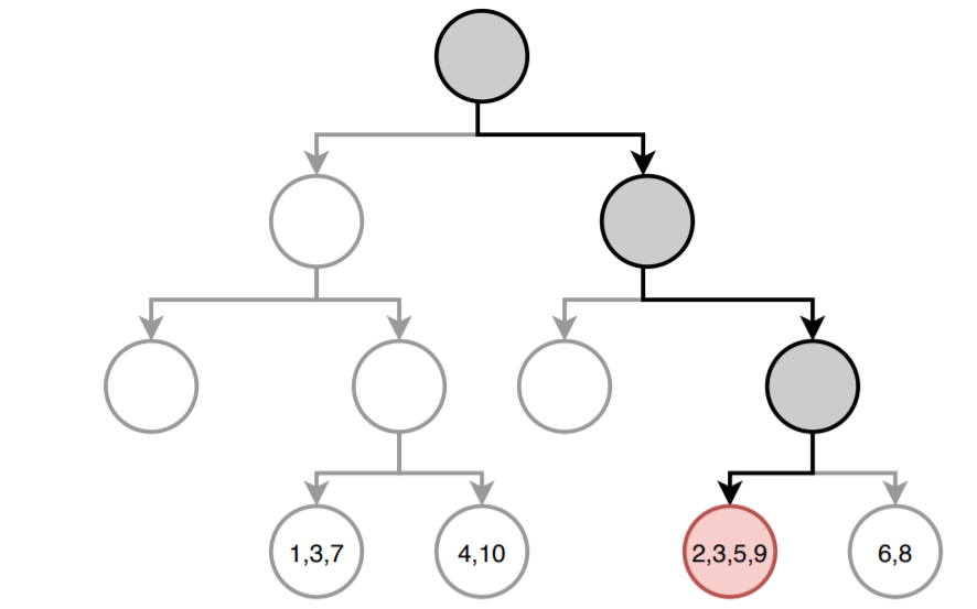
The value predicted by the tree is the mean of the response variable $Y$ of the observations with $id$: 2, 3, 5, 9.
$$\hat{\mu} = \frac{18+24+2+20}{4} = 16$$Although the above is the most common way to obtain predictions from a regression tree, there is another approach. The prediction of a regression tree can be seen as a variant of nearest neighbors where only observations forming part of the same terminal node as the predicted observation have influence. Following this approach, the tree prediction is defined as the weighted mean of all training observations, where the weight of each observation depends solely on whether it is part of the same terminal node or not.
$$\hat{\mu} = \sum^n_{i =1} \textbf{w}_iY_i$$The value of the positions of the weight vector $\textbf{w}$ is $1$ for observations in the same node and $0$ for the rest. In this example it would be:
$$\textbf{w} =(0, 1, 1, 0, 1, 0, 0, 0, 1, 0)$$For the sum of all weights to be $1$, they are divided by the total number of observations in the selected terminal node, in this case 4.
$$\textbf{w} = (0, \frac{1}{4}, \frac{1}{4}, 0, \frac{1}{4}, 0, 0, 0, \frac{1}{4}, 0)$$Thus, the predicted value is:
$$\hat{\mu} = (0\times10) + (\frac{1}{4}\times18) + (\frac{1}{4}\times24) + (0\times8) + (\frac{1}{4}\times2) + \\ (0\times9) + (0\times16) + (0\times10) + (\frac{1}{4}\times20) + (0\times14) = 16$$Classification Trees
Regression trees are the subtype of prediction trees applied when the response variable is categorical.
Tree Construction
To build a classification tree, the same recursive binary splitting method described in regression trees is used. However, since the response variable is qualitative, RSS cannot be used as a criterion for selecting optimal splits. There are several alternatives, all with the goal of finding nodes that are as pure/homogeneous as possible. The most used are:
CLASSIFICATION ERROR RATE
Defined as the proportion of observations that do not belong to the majority class of the node.
$$E_m = 1 - max_k(\hat{p}_{mk})$$where $\hat{p}_{mk}$ represents the proportion of observations in node $m$ belonging to class $k$. Despite the simplicity of this measure, it is not sensitive enough to create good trees, so in practice, it is not usually used.
GINI INDEX
Quantifies the total variance across the $K$ classes of node $m$, that is, it measures the purity of the node.
$$G_m = \sum_{k=1}^K \hat{p}_{mk}(1-\hat{p}_{mk})$$When $\hat{p}_{mk}$ is close to 0 or 1 (the node contains mostly observations of a single class), the term $\hat{p}_{mk}(1-\hat{p}_{mk})$ is very small. Consequently, the higher the purity of the node, the lower the value of the Gini index $G$.
The CART (Classification and Regression Trees) algorithm uses Gini as a splitting criterion.
INFORMATION GAIN: CROSS ENTROPY
Entropy is a way to quantify the disorder of a system. In the case of nodes, disorder corresponds to impurity. If a node is pure, it contains only observations of one class, its entropy is zero. Conversely, if the frequency of each class is the same, the entropy value reaches the maximum value of 1.
$$D = - \displaystyle\sum_{k=1}^K \hat{p}_{mk} \ log(\hat{p}_{mk})$$Algorithms C4.5 and C5.0 use information gain as a splitting criterion.
CHI-SQUARE
This approach consists of identifying if there is a significant difference between child nodes and the parent node, that is, if there is evidence that the split achieves an improvement. To do this, a chi-square goodness of fit statistical test is applied using the frequency of each class in the parent node as the expected distribution $H_0$. The higher the $\chi^2$ statistic, the greater the statistical evidence that there is a difference.
$$\chi^2 = \sum_{k} \frac{(\text{observed}_{k} - \text{expected}_{k})^2}{\text{expected}_{k}}$$Trees generated with this splitting criterion are called CHAID (Chi-square Automatic Interaction Detector).
Regardless of the measure used as a selection criterion for splits, the process is always the same:
For each possible split, the value of the measure is calculated in each of the two resulting nodes.
The two values are summed, weighting each by the fraction of observations contained in each node. This step is very important, since two pure nodes with 2 observations are not the same as two pure nodes with 100 observations.
- The split with the lowest or highest value (depending on the measure used) is selected as the optimal cut point.
For the tree construction process, according to the book Introduction to Statistical Learning, Gini index and cross-entropy are more suitable than classification error rate due to their greater sensitivity to node homogeneity. For the pruning process (described in the next section), all three are suitable, although if the goal is to achieve maximum prediction accuracy, it is better to use classification error rate.
Tree Prediction
After creating a tree, training observations are grouped in terminal nodes. To predict a new observation, the tree is traversed based on the value of its predictors until reaching one of the terminal nodes. In the case of classification, the mode of the response variable is usually used as the prediction value, that is, the most frequent class of the node. Additionally, it can be accompanied by the percentage of each class in the terminal node, which provides information on the confidence of the prediction.
Avoiding Overfitting
The tree construction process described in the previous sections tends to quickly reduce the training error, that is, the model fits the observations used as training very well. As a consequence, overfitting is generated, reducing its predictive capacity when applied to new data. The reason for this behavior lies in the ease with which trees branch out, acquiring complex structures. In fact, if splits are not limited, every tree ends up fitting perfectly to the training observations, creating one terminal node per observation. There are two strategies to prevent the overfitting problem in trees: limiting the tree size (early stopping) and the pruning process (pruning).
Early Stopping
The final size a tree acquires can be controlled by stopping rules that halt node splitting depending on whether certain conditions are met or not. The names of these conditions may vary depending on the software or library used, but they are usually present in all of them.
Minimum observations for split: defines the minimum number of observations a node must have to be split. The higher the value, the less flexible the model.
Minimum terminal node observations: defines the minimum number of observations terminal nodes must have. Its effect is very similar to minimum observations for split.
Maximum tree depth: defines the maximum depth of the tree, understanding maximum depth as the number of splits in the longest branch (descending) of the tree. The lower the value, the less flexible the model.
Maximum number of terminal nodes: defines the maximum number of terminal nodes the tree can have. Once the limit is reached, splits stop. Its effect is similar to controlling the maximum tree depth.
Minimum error reduction: defines the minimum error reduction a split must achieve to be carried out.
All these parameters are known as hyperparameters because they are not learned during model training. Their value must be specified by the user based on their knowledge of the problem and through the use of validation strategies.
Tree Pruning
The strategy of controlling tree size using stopping rules has a drawback: the tree grows by selecting the best split at each moment. By evaluating splits without considering what will come after, the option resulting in the best final tree is never chosen, unless it is also the one generating the best split at that moment. These types of strategies are known as greedy. An example illustrating the problem of this type of strategy is as follows: suppose a car is driving in the left lane of a two-lane road in the same direction. In the current lane, there are many cars driving at 100 km/h, while the other lane is empty. At a certain distance, a vehicle is observed driving in the right lane at 20 km/h. If the driver's goal is to reach their destination as soon as possible, they have two options: change lanes or stay in the current one. A greedy approach would evaluate the situation at that instant and determine that the best option is to change lanes and accelerate to over 100 km/h; however, in the long run, this is not the best solution, as once they reach the slow vehicle, they will have to reduce their speed significantly.
A non-greedy alternative that avoids overfitting consists of generating large trees, without stopping conditions beyond those necessary due to computational limitations, and then pruning them (pruning), keeping only the robust structure that achieves a low test error. The selection of the optimal sub-tree can be done using cross-validation; however, since trees are grown as much as possible (they have many terminal nodes), it is usually not feasible to estimate the test error of all possible sub-structures that can be generated. Instead, cost complexity pruning or weakest link pruning is used.
Cost complexity pruning is a Loss + Penalty type penalization method, similar to that used in ridge regression or lasso. In this case, the sub-tree $T$ that minimizes the equation is sought:
$$\displaystyle\sum_{j=1}^{|T|} \displaystyle\sum_{i \in R_j}(y_i -\hat{y}_{R_j})^2 + \alpha|T| $$where $|T|$ is the number of terminal nodes in the tree.
The first term of the equation corresponds to the total sum of squared residuals RSS. By definition, the more terminal nodes the model has, the smaller this part of the equation will be. The second term is the constraint, which penalizes the model based on the number of terminal nodes (the higher the number, the greater the penalty). The degree of penalty is determined by the tuning parameter $\alpha$. When $\alpha = 0$, the penalty is null and the resulting tree is equivalent to the original tree. As $\alpha$ increases, the penalty is greater and, consequently, the resulting trees are smaller. The optimal value of $\alpha$ can be identified using cross validation.
Algorithm to create a regression tree with pruning
Recursive binary splitting is used to create a large and complex tree ($T_o$) using the training data and reducing stopping conditions as much as possible. Usually, the only stopping condition used is the minimum number of observations per terminal node.
Cost complexity pruning is applied to the tree $T_o$ to obtain the best sub-tree as a function of $\alpha$. That is, the best sub-tree is obtained for a range of $\alpha$ values.
Identification of the optimal $\alpha$ value using k-cross-validation. The training set is divided into $K$ groups. For $k=1$, ..., $k=K$:
Repeat steps 1 and 2 using all observations except those in group $k_i$.
Evaluate the mean squared error for the range of $\alpha$ values using group $k_i$.
Obtain the average of the $K$ mean squared error calculated for each $\alpha$ value.
Select the sub-tree from step 2 corresponding to the $\alpha$ value that achieved the lowest cross-validation mean squared error in step 3.
In the case of classification trees, instead of using the sum of squared residuals as a selection criterion, one of the homogeneity measures seen in previous sections is used.
Regression Example
Libraries
The libraries used in this example are:
# Data treatment
# ==============================================================================
import numpy as np
import pandas as pd
# Graphics
# ==============================================================================
import matplotlib.pyplot as plt
# Preprocessing and modeling
# ==============================================================================
from sklearn.model_selection import train_test_split
from sklearn.tree import DecisionTreeRegressor
from sklearn.tree import plot_tree
from sklearn.tree import export_text
from sklearn.model_selection import GridSearchCV
from sklearn.metrics import root_mean_squared_error
# Warnings configuration
# ==============================================================================
import warnings
warnings.filterwarnings('once')
Data
The Boston dataset contains housing prices in the city of Boston, as well as socio-economic information about the neighborhood where they are located. The goal is to fit a regression model that allows predicting the average price of a house (MEDV) based on the available variables.
Number of instances: 506
Number of attributes: 13 numeric/categorical predictors.
Attribute information (in order):
- CRIM: per capita crime rate by town.
- ZN: proportion of residential land zoned for lots over 25,000 sq.ft.
- INDUS: proportion of non-retail business acres per town.
- CHAS: Charles River dummy variable (= 1 if tract bounds river; 0 otherwise).
- NOX: nitric oxides concentration (parts per 10 million).
- RM: average number of rooms per dwelling.
- AGE: proportion of owner-occupied units built prior to 1940.
- DIS: weighted distances to five Boston employment centres.
- RAD: index of accessibility to radial highways.
- TAX: full-value property-tax rate per $10,000.
- PTRATIO: pupil-teacher ratio by town.
- LSTAT: % lower status of the population.
- MEDV: Median value of owner-occupied homes in $1000's.
Missing values: None
# Data download
# ==============================================================================
url = (
'https://raw.githubusercontent.com/JoaquinAmatRodrigo/Estadistica-machine-learning-python/'
'master/data/Boston.csv'
)
data = pd.read_csv(url, sep=',')
display(data.head(3))
display(data.info())
| CRIM | ZN | INDUS | CHAS | NOX | RM | AGE | DIS | RAD | TAX | PTRATIO | LSTAT | MEDV | |
|---|---|---|---|---|---|---|---|---|---|---|---|---|---|
| 0 | 0.00632 | 18.0 | 2.31 | 0 | 0.538 | 6.575 | 65.2 | 4.0900 | 1 | 296 | 15.3 | 4.98 | 24.0 |
| 1 | 0.02731 | 0.0 | 7.07 | 0 | 0.469 | 6.421 | 78.9 | 4.9671 | 2 | 242 | 17.8 | 9.14 | 21.6 |
| 2 | 0.02729 | 0.0 | 7.07 | 0 | 0.469 | 7.185 | 61.1 | 4.9671 | 2 | 242 | 17.8 | 4.03 | 34.7 |
<class 'pandas.core.frame.DataFrame'> RangeIndex: 506 entries, 0 to 505 Data columns (total 13 columns): # Column Non-Null Count Dtype --- ------ -------------- ----- 0 CRIM 506 non-null float64 1 ZN 506 non-null float64 2 INDUS 506 non-null float64 3 CHAS 506 non-null int64 4 NOX 506 non-null float64 5 RM 506 non-null float64 6 AGE 506 non-null float64 7 DIS 506 non-null float64 8 RAD 506 non-null int64 9 TAX 506 non-null int64 10 PTRATIO 506 non-null float64 11 LSTAT 506 non-null float64 12 MEDV 506 non-null float64 dtypes: float64(10), int64(3) memory usage: 51.5 KB
None
Model Fitting
The DecisionTreeRegressor class from the sklearn.tree module allows training decision trees for regression problems. Below, a regression tree is fitted using MEDV as the response variable and all other available variables as predictors.
DecisionTreeRegressor has the following default hyperparameters:
criterion='squared_error'splitter='best'max_depth=Nonemin_samples_split=2min_samples_leaf=1min_weight_fraction_leaf=0.0max_features=Nonerandom_state=Nonemax_leaf_nodes=Nonemin_impurity_decrease=0.0min_impurity_split=Noneccp_alpha=0.0monotonic_cst
Among all of them, the most important are those that stop the tree growth (stop conditions):
max_depth: maximum depth the tree can reach.min_samples_split: minimum number of observations a node must have to be split. If it is a decimal value, it is interpreted as a fraction of the total training observationsceil(min_samples_split * n_samples).min_samples_leaf: minimum number of observations each child node must have for the split to occur. If it is a decimal value, it is interpreted as a fraction of the total training observationsceil(min_samples_split * n_samples).max_leaf_nodes: maximum number of terminal nodes.random_state: seed for reproducibility. Must be an integer value.
As in any regression study, it is not only important to fit the model, but also to quantify its ability to predict new observations. To perform the subsequent evaluation, the data is divided into two groups, one for training and one for testing.
# Split data into train and test
# ==============================================================================
X_train, X_test, y_train, y_test = train_test_split(
data.drop(columns = "MEDV"),
data['MEDV'],
random_state = 123
)
# Model creation
# ==============================================================================
model = DecisionTreeRegressor(max_depth=3, random_state=123)
# Model training
# ==============================================================================
model.fit(X_train, y_train)
DecisionTreeRegressor(max_depth=3, random_state=123)In a Jupyter environment, please rerun this cell to show the HTML representation or trust the notebook.
On GitHub, the HTML representation is unable to render, please try loading this page with nbviewer.org.
Parameters
| criterion | 'squared_error' | |
| splitter | 'best' | |
| max_depth | 3 | |
| min_samples_split | 2 | |
| min_samples_leaf | 1 | |
| min_weight_fraction_leaf | 0.0 | |
| max_features | None | |
| random_state | 123 | |
| max_leaf_nodes | None | |
| min_impurity_decrease | 0.0 | |
| ccp_alpha | 0.0 | |
| monotonic_cst | None |
Once the tree is trained, it can be represented using the combination of plot_tree() and export_text() functions. The plot_tree() function draws the tree structure and shows the number of observations and mean value of the response variable in each node. The export_text() function represents this same information in text format.
# Structure of the created tree
# ==============================================================================
fig, ax = plt.subplots(figsize=(9, 5))
print(f"Tree depth: {model.get_depth()}")
print(f"Number of terminal nodes: {model.get_n_leaves()}")
plot = plot_tree(
decision_tree = model,
feature_names = data.drop(columns = "MEDV").columns,
class_names = ['MEDV'],
filled = True,
impurity = False,
fontsize = 8,
precision = 2,
ax = ax
)
Profundidad del árbol: 3 Número de nodos terminales: 8

# Structure in text format
# ==============================================================================
model_text = export_text(
decision_tree = model,
feature_names = list(data.drop(columns = "MEDV").columns)
)
print(model_text)
|--- RM <= 6.98 | |--- LSTAT <= 14.39 | | |--- DIS <= 1.42 | | | |--- value: [50.00] | | |--- DIS > 1.42 | | | |--- value: [23.13] | |--- LSTAT > 14.39 | | |--- CRIM <= 6.99 | | | |--- value: [16.96] | | |--- CRIM > 6.99 | | | |--- value: [11.58] |--- RM > 6.98 | |--- RM <= 7.44 | | |--- DIS <= 1.57 | | | |--- value: [50.00] | | |--- DIS > 1.57 | | | |--- value: [32.17] | |--- RM > 7.44 | | |--- PTRATIO <= 17.90 | | | |--- value: [47.36] | | |--- PTRATIO > 17.90 | | | |--- value: [40.12]
Following the leftmost branch of the tree, it can be seen that the model predicts an average price of 50,000 dollars for houses located in an area with RM <= 6.98, LSTAT <= 14.39 and DIS <= 1.42.
Feature Importance
The importance of each predictor in the model is calculated as the total reduction (normalized) in the splitting criterion, in this case mse, achieved by the predictor in the splits in which it participates. If a predictor has not been selected in any split, it has not been included in the model and therefore its importance is 0.
feature_importance = pd.DataFrame(
{
"predictor": data.drop(columns="MEDV").columns,
"importance": model.feature_importances_,
}
)
print("Importance of predictors in the model")
print("-------------------------------------------")
feature_importance.sort_values("importance", ascending=False)
Importancia de los predictores en el modelo -------------------------------------------
| predictor | importancia | |
|---|---|---|
| 5 | RM | 0.671680 |
| 11 | LSTAT | 0.222326 |
| 7 | DIS | 0.064816 |
| 0 | CRIM | 0.034714 |
| 10 | PTRATIO | 0.006465 |
| 3 | CHAS | 0.000000 |
| 1 | ZN | 0.000000 |
| 2 | INDUS | 0.000000 |
| 6 | AGE | 0.000000 |
| 4 | NOX | 0.000000 |
| 9 | TAX | 0.000000 |
| 8 | RAD | 0.000000 |
The predictor RM, the average number of rooms in the houses of the area, has turned out to be the most important predictor in the model, followed by LSTAT, which measures the percentage of people in poverty.
Tree Pruning
In order to reduce the variance of the model and thus improve predictive capacity, the tree is subjected to a pruning process. As described previously, the pruning process attempts to find the simplest tree (smallest size) that achieves the best prediction results.
To apply the pruning process, it is necessary to indicate the ccp_alpha argument which determines the degree of complexity penalty. The higher this value, the more aggressive the pruning and the smaller the resulting tree size. Since there is no way to know the optimal value of ccp_alpha beforehand, cross-validation is used to identify it.
Although there are other ways to identify "optimal" trees, for example by identifying the value of max_depth and min_samples_split through cross-validation, pruning can generate better results as it allows a less useful split to be maintained if the subsequent splits starting from it are useful.
# Pruning (cost complexity pruning) by cross-validation
# ==============================================================================
# Values of ccp_alpha evaluated
param_grid = {'ccp_alpha': np.linspace(0, 20, 20)}
# Search by cross-validation
grid = GridSearchCV(
# The tree is grown to the maximum possible before applying pruning
estimator = DecisionTreeRegressor(
max_depth = None,
min_samples_split = 2,
min_samples_leaf = 1,
random_state = 123
),
param_grid = param_grid,
scoring = 'neg_mean_squared_error',
cv = 10,
refit = True,
return_train_score = True
)
grid.fit(X_train, y_train)
fig, ax = plt.subplots(figsize=(8, 3.84))
scores = pd.DataFrame(grid.cv_results_)
# Convert to positive error for easier reading (MSE)
scores['mean_train_score'] = -scores['mean_train_score']
scores['mean_test_score'] = -scores['mean_test_score']
scores.plot(x='param_ccp_alpha', y='mean_train_score', yerr='std_train_score', ax=ax, marker='o', label='Train Error')
scores.plot(x='param_ccp_alpha', y='mean_test_score', yerr='std_test_score', ax=ax, marker='o', label='CV Error')
# Mark the best alpha
best_alpha = grid.best_params_['ccp_alpha']
ax.axvline(x=best_alpha, color='red', linestyle='--', label=f'Best alpha: {best_alpha:.2f}')
ax.set_title("Cross-validation error (MSE) vs ccp_alpha hyperparameter")
ax.set_ylabel("Mean Squared Error")
ax.legend();

# Best ccp_alpha value found
# ==============================================================================
grid.best_params_
{'ccp_alpha': np.float64(1.0526315789473684)}
Once the optimal value of ccp_alpha is identified, the tree is retrained indicating this value in its arguments. If refit=True is indicated in GridSearchCV(), this retraining is done automatically and the resulting model is stored in .best_estimator_.
# Structure of the final tree
# ==============================================================================
final_model = grid.best_estimator_
print(f"Tree depth: {final_model.get_depth()}")
print(f"Number of terminal nodes: {final_model.get_n_leaves()}")
fig, ax = plt.subplots(figsize=(7, 5))
plot = plot_tree(
decision_tree = final_model,
feature_names = data.drop(columns = "MEDV").columns,
class_names = ['MEDV'],
filled = True,
impurity = False,
ax = ax
)
Profundidad del árbol: 4 Número de nodos terminales: 7

Model Prediction and Evaluation
Finally, the predictive capacity of the final tree is evaluated using the test set.
# Test error of the final model (after applying pruning)
# ==============================================================================
predictions = final_model.predict(X = X_test)
rmse = root_mean_squared_error(
y_true = y_test,
y_pred = predictions,
)
print(f"The test error (rmse) is: {rmse}")
El error (rmse) de test es: 5.522220519181609
The pruning process has generated a tree with a depth of 4 and 7 terminal nodes. The predictions of the final model deviate on average 5.52 units (5520 dollars) from the real value.
Classification Example
Libraries
The libraries used in this example are:
# Data treatment
# ==============================================================================
import numpy as np
import pandas as pd
import statsmodels.api as sm
# Graphics
# ==============================================================================
import matplotlib.pyplot as plt
# Preprocessing and modeling
# ==============================================================================
from sklearn.model_selection import train_test_split
from sklearn.tree import DecisionTreeClassifier
from sklearn.tree import plot_tree
from sklearn.tree import export_text
from sklearn.model_selection import GridSearchCV
from sklearn.compose import ColumnTransformer
from sklearn.preprocessing import OneHotEncoder
from sklearn.metrics import (
accuracy_score,
classification_report,
confusion_matrix,
ConfusionMatrixDisplay,
)
# Warnings configuration
# ==============================================================================
import warnings
warnings.filterwarnings("ignore")
Data
The Carseats dataset, originally from the R package ISLR and accessible in Python through statsmodels.datasets.get_rdataset, contains information on the sale of child car seats in 400 different stores. For each of the 400 stores, 11 variables have been recorded. The goal is to generate a classification model that allows predicting whether a store has high sales (Sales > 8) or low sales (Sales <= 8) based on all available variables.
💡 Tip
You can find a list of all available datasets at Rdatasets
# Data download
# ==============================================================================
carseats = sm.datasets.get_rdataset("Carseats", "ISLR")
data = carseats.data
# print(carseats.__doc__)
data.head(3)
| Sales | CompPrice | Income | Advertising | Population | Price | ShelveLoc | Age | Education | Urban | US | |
|---|---|---|---|---|---|---|---|---|---|---|---|
| 0 | 9.50 | 138 | 73 | 11 | 276 | 120 | Bad | 42 | 17 | Yes | Yes |
| 1 | 11.22 | 111 | 48 | 16 | 260 | 83 | Good | 65 | 10 | Yes | Yes |
| 2 | 10.06 | 113 | 35 | 10 | 269 | 80 | Medium | 59 | 12 | Yes | Yes |
Since Sales is a continuous variable and the goal of the study is to classify stores according to whether they sell a lot or a little, a new dichotomous variable (0, 1) called high_sales is created.
data['high_sales'] = np.where(data.Sales > 8, 1, 0)
# Once the new response variable is created, the original one is discarded
data = data.drop(columns = 'Sales')
data.head(3)
| CompPrice | Income | Advertising | Population | Price | ShelveLoc | Age | Education | Urban | US | ventas_altas | |
|---|---|---|---|---|---|---|---|---|---|---|---|
| 0 | 138 | 73 | 11 | 276 | 120 | Bad | 42 | 17 | Yes | Yes | 1 |
| 1 | 111 | 48 | 16 | 260 | 83 | Good | 65 | 10 | Yes | Yes | 1 |
| 2 | 113 | 35 | 10 | 269 | 80 | Medium | 59 | 12 | Yes | Yes | 1 |
Model Fitting
A classification tree is fitted using high_sales as the response variable and all available variables as predictors. First, the hyperparameters max_depth=5 and criterion='gini' are used, the rest are left as default. Then, the pruning process is applied and the results are compared against the initial model.
Unlike the previous example, these data contain categorical variables, so before training the model, it is necessary to apply one-hot-encoding. A more detailed description of this process can be found in Machine Learning with Python and Scikit-learn.
# Split data into train and test
# ==============================================================================
X_train, X_test, y_train, y_test = train_test_split(
data.drop(columns = 'high_sales'),
data['high_sales'],
random_state = 123
)
# One-hot-encoding of categorical variables
# ==============================================================================
# Identify the name of numeric and categorical columns
cat_cols = X_train.select_dtypes(include=['object', 'category']).columns.to_list()
numeric_cols = X_train.select_dtypes(include=['float64', 'int']).columns.to_list()
# Apply one-hot-encoding only to categorical columns
preprocessor = ColumnTransformer(
[('onehot', OneHotEncoder(handle_unknown='ignore', sparse_output=False, dtype=float), cat_cols)],
remainder='passthrough',
verbose_feature_names_out=False
).set_output(transform='pandas')
# Once the ColumnTransformer object is defined, with the fit() method
# transformations are learned with the training data and applied to
# both sets with transform(). Both operations at once with fit_transform().
X_train_prep = preprocessor.fit_transform(X_train)
X_test_prep = preprocessor.transform(X_test)
X_train_prep.info()
<class 'pandas.core.frame.DataFrame'> Index: 300 entries, 170 to 365 Data columns (total 14 columns): # Column Non-Null Count Dtype --- ------ -------------- ----- 0 ShelveLoc_Bad 300 non-null float64 1 ShelveLoc_Good 300 non-null float64 2 ShelveLoc_Medium 300 non-null float64 3 Urban_No 300 non-null float64 4 Urban_Yes 300 non-null float64 5 US_No 300 non-null float64 6 US_Yes 300 non-null float64 7 CompPrice 300 non-null int64 8 Income 300 non-null int64 9 Advertising 300 non-null int64 10 Population 300 non-null int64 11 Price 300 non-null int64 12 Age 300 non-null int64 13 Education 300 non-null int64 dtypes: float64(7), int64(7) memory usage: 35.2 KB
# Model creation
# ==============================================================================
model = DecisionTreeClassifier(
max_depth = 5,
criterion = 'gini',
random_state = 123
)
# Model training
# ==============================================================================
model.fit(X_train_prep, y_train)
DecisionTreeClassifier(max_depth=5, random_state=123)In a Jupyter environment, please rerun this cell to show the HTML representation or trust the notebook.
On GitHub, the HTML representation is unable to render, please try loading this page with nbviewer.org.
Parameters
| criterion | 'gini' | |
| splitter | 'best' | |
| max_depth | 5 | |
| min_samples_split | 2 | |
| min_samples_leaf | 1 | |
| min_weight_fraction_leaf | 0.0 | |
| max_features | None | |
| random_state | 123 | |
| max_leaf_nodes | None | |
| min_impurity_decrease | 0.0 | |
| class_weight | None | |
| ccp_alpha | 0.0 | |
| monotonic_cst | None |
# Structure of the created tree
# ==============================================================================
fig, ax = plt.subplots(figsize=(10, 6))
print(f"Tree depth: {model.get_depth()}")
print(f"Number of terminal nodes: {model.get_n_leaves()}")
plot = plot_tree(
decision_tree = model,
feature_names = X_train_prep.columns.to_list(),
class_names = y_train.unique().astype(str).tolist(),
filled = True,
impurity = False,
fontsize = 6,
ax = ax
)
Profundidad del árbol: 5 Número de nodos terminales: 23

Model Prediction and Evaluation
The predictive capacity of the initial tree is evaluated by calculating the accuracy on the test set.
# Predictions on the test set
# ==============================================================================
predictions = model.predict(X=X_test_prep)
print(predictions)
[1 0 1 1 1 0 0 1 0 0 0 0 0 1 0 0 1 0 0 0 0 0 1 1 0 0 1 0 0 0 0 0 0 1 1 0 0 0 0 1 0 0 0 1 0 1 1 0 0 0 0 0 0 1 0 1 1 0 0 1 0 0 0 0 1 1 1 0 0 1 0 0 0 0 1 0 0 0 0 0 1 0 0 0 0 1 0 1 0 0 1 0 1 0 1 1 0 0 1 0]
# Model test error
# ==============================================================================
print("Confusion Matrix")
print("-------------------")
cm = confusion_matrix(y_true=y_test, y_pred=predictions)
disp = ConfusionMatrixDisplay(confusion_matrix=cm, display_labels=model.classes_)
disp.plot();
Matriz de confusión -------------------

# Classification report
# ==============================================================================
print(classification_report(y_true=y_test, y_pred=predictions))
precision recall f1-score support
0 0.66 0.88 0.75 50
1 0.82 0.54 0.65 50
accuracy 0.71 100
macro avg 0.74 0.71 0.70 100
weighted avg 0.74 0.71 0.70 100
The initial model is able to correctly predict 71% of the observations in the test set.
Tree Pruning
Although a value of max_depth=5 was initially used, this does not have to be the best value. With the aim of identifying the optimal depth that manages to reduce variance and increase the predictive capacity of the model, the tree is subjected to a pruning process.
# Post pruning (cost complexity pruning) by cross-validation
# ==============================================================================
# Values of ccp_alpha evaluated
param_grid = {'ccp_alpha':np.linspace(0, 5, 10)}
# Search by cross-validation
grid = GridSearchCV(
# The tree is grown to the maximum possible before applying pruning
estimator = DecisionTreeClassifier(
max_depth = None,
min_samples_split = 2,
min_samples_leaf = 1,
random_state = 123
),
param_grid = param_grid,
scoring = 'accuracy',
cv = 10,
refit = True,
return_train_score = True
)
grid.fit(X_train_prep, y_train)
fig, ax = plt.subplots(figsize=(8, 3.84))
scores = pd.DataFrame(grid.cv_results_)
scores.plot(x='param_ccp_alpha', y='mean_train_score', yerr='std_train_score', ax=ax)
scores.plot(x='param_ccp_alpha', y='mean_test_score', yerr='std_test_score', ax=ax)
ax.set_title("Cross-validation error vs ccp_alpha hyperparameter");

# Best ccp_alpha value found
# ==============================================================================
grid.best_params_
{'ccp_alpha': np.float64(0.0)}
Once the optimal value of ccp_alpha is identified, the tree is retrained indicating this value in its arguments. If refit=True is indicated in GridSearchCV(), this retraining is done automatically and the resulting model is stored in .best_estimator_.
# Structure of the final tree
# ==============================================================================
final_model = grid.best_estimator_
print(f"Tree depth: {final_model.get_depth()}")
print(f"Number of terminal nodes: {final_model.get_n_leaves()}")
Profundidad del árbol: 9 Número de nodos terminales: 49
# Test error of the final model
# ==============================================================================
predictions = final_model.predict(X = X_test_prep)
accuracy = accuracy_score(
y_true = y_test,
y_pred = predictions,
normalize = True
)
print(f"The test accuracy is: {100 * accuracy} %")
El accuracy de test es: 75.0 %
Thanks to the pruning process, the accuracy percentage has gone from 71% to 75%.
Feature Importance
The importance of each predictor in the model is calculated as the total reduction (normalized) in the splitting criterion, in this case the Gini index, achieved by the predictor in the splits in which it participates. If a predictor has not been selected in any split, it has not been included in the model and therefore its importance is 0.
print("Importance of predictors in the model")
print("-------------------------------------------")
feature_importance = pd.DataFrame(
{'predictor': final_model.feature_names_in_,
'importance': final_model.feature_importances_}
)
feature_importance.sort_values('importance', ascending=False)
Importancia de los predictores en el modelo -------------------------------------------
| predictor | importancia | |
|---|---|---|
| 11 | Price | 0.267291 |
| 7 | CompPrice | 0.173585 |
| 1 | ShelveLoc_Good | 0.163736 |
| 8 | Income | 0.093583 |
| 9 | Advertising | 0.089938 |
| 12 | Age | 0.055480 |
| 6 | US_Yes | 0.039439 |
| 4 | Urban_Yes | 0.035371 |
| 0 | ShelveLoc_Bad | 0.033437 |
| 10 | Population | 0.024170 |
| 5 | US_No | 0.012651 |
| 13 | Education | 0.011319 |
| 2 | ShelveLoc_Medium | 0.000000 |
| 3 | Urban_No | 0.000000 |
Probability Prediction
Most implementations of tree-based models, including scikit-learn, allow predicting probabilities when dealing with classification problems. It is important to understand how these values are calculated to interpret and use them correctly.
In the previous example, applying .predict() returns $1$ (high sales) or $0$ (low sales) for each test observation. However, there is no information about the certainty with which the model makes this assignment. With .predict_proba(), instead of a classification, the probability with which the model considers that each observation may belong to each of the classes is obtained.
# Probability prediction
# ==============================================================================
predictions = model.predict_proba(X = X_test_prep)
predictions[:5, :]
array([[0. , 1. ],
[1. , 0. ],
[0.10526316, 0.89473684],
[0.05555556, 0.94444444],
[0.10526316, 0.89473684]])
The result of .predict_proba() is an array with one row per observation and as many columns as classes the response variable has. The value of the first column corresponds to the probability, according to the model, that the observation belongs to class 0, and so on. The probability value shown for each prediction corresponds to the fraction of observations of each class in the terminal node reached by the predicted observation.
By default, .predict() assigns each new observation to the class with the highest probability (in case of a tie, it is assigned randomly). However, this does not have to be the desired behavior in all cases.
# Classification using the class with the highest probability
# ==============================================================================
predictions_df = pd.DataFrame(data=predictions, columns=['0', '1'])
predictions_df['classification_default_0.5'] = np.where(predictions_df['0'] > predictions_df['1'], 0, 1)
predictions_df.head(3)
| 0 | 1 | clasificacion_default_0.5 | |
|---|---|---|---|
| 0 | 0.000000 | 1.000000 | 1 |
| 1 | 1.000000 | 0.000000 | 0 |
| 2 | 0.105263 | 0.894737 | 1 |
Suppose the following scenario: the Christmas campaign is approaching and the chain owners want to double the stock of items in those stores that are predicted to have high sales. Since transporting this material to the stores involves a high cost, the director wants to limit this strategy only to stores for which there is high certainty that they will achieve high sales.
If probabilities are available, a specific cut-off point can be established, for example, considering only as class $1$ (high sales) those stores whose prediction for this class is greater than 0.8 (80%). In this way, the final classification better fits the needs of the use case.
# Final classification using a threshold of 0.8 for class 1.
# ==============================================================================
predictions_df['classification_custom_0.8'] = np.where(predictions_df['1'] > 0.8, 1, 0)
predictions_df.iloc[5:10, :]
| 0 | 1 | clasificacion_default_0.5 | clasificacion_custom_0.8 | |
|---|---|---|---|---|
| 5 | 0.500000 | 0.500000 | 1 | 0 |
| 6 | 0.928571 | 0.071429 | 0 | 0 |
| 7 | 0.055556 | 0.944444 | 1 | 1 |
| 8 | 0.985507 | 0.014493 | 0 | 0 |
| 9 | 0.708333 | 0.291667 | 0 | 0 |
To what extent should these probabilities be trusted?
It is very important to keep in mind the difference between the model's view of the world and the real world. Everything a model knows about the real world is what it has been able to learn from the training data and, therefore, it has a limited view. For example, suppose that in the training data, all stores in an urban area Urban='Yes' have high sales regardless of the value of the other predictors. When the model tries to predict a new observation, if it is in an urban area, it will classify the store as high sales with 100% certainty. However, this does not mean that it is unequivocally true; there could be stores in urban areas that do not have high sales but, not being present in the training data, the model does not contemplate this possibility.
Another example of how these probabilities can be misleading is the following. If a tree is allowed to grow until all training observations are in a different terminal node, when a new prediction is made, regardless of the node it ends up in, 100% of the observations (there is only one) will belong to the same class. Since the probability value is the percentage of observations belonging to each class in the terminal node, the model will always predict with 100% probability even if it is wrong.
Taking all this into account, the probabilities generated by the model should be considered as the certainty it has, from its limited view, when making predictions. But not as the probability in the real world that this is the case.
Comparison of Trees vs Linear Models
The superiority of decision tree-based methods over linear methods depends on the problem at hand. When the relationship between predictors and the response variable is approximately linear, a linear regression type model works well and outperforms regression trees.
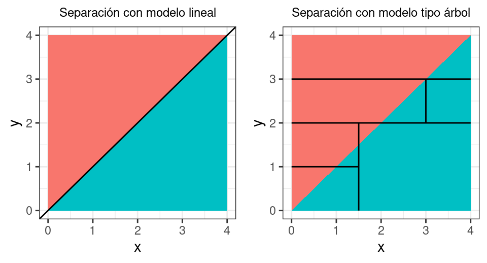
Conversely, if the relationship between predictors and the response variable is non-linear and complex, tree-based methods usually outperform classical linear approaches.
Dummy Variables (one-hot-encoding) in Tree Models
Decision tree-based models are capable of using categorical predictors in their natural form without the need to convert them into dummy variables using one-hot-encoding. However, in practice, it depends on the implementation of the library or software used. This has a direct impact on the structure of the generated trees and, consequently, on the predictive results of the model and the importance calculated for the predictors.
In the book Feature Engineering and Selection A Practical Approach for Predictive Models By Max Kuhn, Kjell Johnson, the authors perform an experiment comparing models trained with and without one-hot-encoding on 5 different datasets, the results show that:
There is no clear difference in terms of predictive capacity of the models. Only in the case of stochastic gradient boosting are slight differences appreciated against applying one-hot-encoding.
Model training takes on average 2.5 times longer when one-hot-encoding is applied. This is due to the increase in dimensionality by creating the new dummy variables, forcing the algorithm to analyze many more split points.
Based on the results obtained, the authors recommend not applying one-hot-encoding. Only if the results are good, then test if they improve by creating dummy variables.
Another detailed comparison can be found in Are categorical variables getting lost in your random forests? By Nick Dingwall, Chris Potts, where the results show that:
When converting a categorical variable into multiple dummy variables, its importance is diluted, making it difficult for the model to learn from it and thus losing predictive capacity. This effect is greater the more levels the original variable has.
By diluting the importance of categorical predictors, they are less likely to be selected by the model, which distorts the metrics measuring predictor importance.
For the moment, in scikit-learn it is necessary to do one-hot-encoding to convert categorical variables into dummy variables.
Extrapolation with Tree Models
An important limitation of regression trees is that they do not extrapolate outside the training range. When the model is applied to a new observation whose predictor value or values are higher or lower than those observed in training, the prediction is always the mean of the closest node, regardless of how far the value is. See the following example where two models are trained, a linear model and a regression tree, and then values of $X$ outside the training range are predicted.
import matplotlib.pyplot as plt
import numpy as np
from sklearn.tree import DecisionTreeRegressor
from sklearn.linear_model import LinearRegression
# Simulated data
# ==============================================================================
X = np.linspace(0, 150, 100)
y = (X + 100) + np.random.normal(loc=0.0, scale=5.0, size=X.shape)
X_train = X[(X>=50) & (X<100)]
y_train = y[(X>=50) & (X<100)]
X_test_lower = X[X < 50]
y_test_lower = y[X < 50]
X_test_upper = X[X >= 100]
y_test_upper = y[X >= 100]
fig, ax = plt.subplots(figsize=(7, 4))
ax.plot(X_train, y_train, c='black', linestyle='dashed', label = "Train data")
ax.axvspan(50, 100, color='gray', alpha=0.2, lw=0)
ax.plot(X_test_lower, y_test_lower, c='blue', linestyle='dashed', label = "Test data")
ax.plot(X_test_upper, y_test_upper, c='blue', linestyle='dashed')
ax.set_title("Train and Test Data")
plt.legend();

# Linear model
linear_model = LinearRegression()
linear_model.fit(X_train.reshape(-1, 1), y_train)
# Tree model
tree_model = DecisionTreeRegressor(max_depth=4)
tree_model.fit(X_train.reshape(-1, 1), y_train)
# Predictions
linear_prediction = linear_model.predict(X.reshape(-1, 1))
tree_prediction = tree_model.predict(X.reshape(-1, 1))
fig, ax = plt.subplots(figsize=(7, 4))
ax.plot(X_train, y_train, c='black', linestyle='dashed', label = "Train data")
ax.axvspan(50, 100, color='gray', alpha=0.2, lw=0)
ax.plot(X_test_lower, y_test_lower, c='blue', linestyle='dashed', label = "Test data")
ax.plot(X_test_upper, y_test_upper, c='blue', linestyle='dashed')
ax.plot(X, linear_prediction, c='firebrick',
label = "Linear model prediction")
ax.plot(X, tree_prediction, c='orange',
label = "Tree model prediction")
ax.set_title("Extrapolation of a linear model and a tree model")
plt.legend();

The graph shows that, with the tree model, the predicted value outside the training range is the same regardless of how far X moves away. A strategy that allows trees to extrapolate is to fit a linear model in each terminal node, but it is not available in Scikit-learn.
Bibliography
Introduction to Statistical Learning, Gareth James, Daniela Witten, Trevor Hastie and Robert Tibshirani
Applied Predictive Modeling Max Kuhn, Kjell Johnson
T.Hastie, R.Tibshirani, J.Friedman. The Elements of Statistical Learning. Springer, 2009
Bradley Efron and Trevor Hastie. 2016. Computer Age Statistical Inference: Algorithms, Evidence, and Data Science (1st. ed.). Cambridge University Press, USA.
Scikit-learn: Machine Learning in Python, Pedregosa et al., JMLR 12, pp. 2825-2830, 2011.
API design for machine learning software: experiences from the scikit-learn project, Buitinck et al., 2013.
Citation Instructions
How to cite this document?
If you use this document or any part of it, we appreciate you citing it. Thank you very much!
Decision Trees with Python: Regression and Classification by Joaquín Amat Rodrigo, available under an Attribution-NonCommercial-ShareAlike 4.0 International (CC BY-NC-SA 4.0 DEED) license at https://www.cienciadedatos.net/documentos/py07-decision-trees-python.html
Did you like the article? Your help is important
Your contribution will help me continue generating free educational content. Thank you very much! 😊


This document created by Joaquín Amat Rodrigo is licensed under Attribution-NonCommercial-ShareAlike 4.0 International.
Allowed:
-
Share: copy and redistribute the material in any medium or format.
-
Adapt: remix, transform, and build upon the material.
Under the following terms:
-
Attribution: You must give appropriate credit, provide a link to the license, and indicate if changes were made. You may do so in any reasonable manner, but not in any way that suggests the licensor endorses you or your use.
-
Non-Commercial: You may not use the material for commercial purposes.
-
ShareAlike: If you remix, transform, or build upon the material, you must distribute your contributions under the same license as the original.