More about machine learning: Machine Learning with Python
- Linear regression
- Logistic regression
- Decision trees
- Random forest
- Gradient boosting
- Machine learning with Python and Scikitlearn
- Neural Networks
- Principal Component Analysis (PCA)
- Clustering with python
- Anomaly detection with PCA
- Face Detection and Recognition
- Introduction to Graphs and Networks
Introduction
Principal Component Analysis (PCA) is a dimensionality reduction method that allows you to simplify the complexity of multi-dimensional spaces while preserving their information.
Suppose you have a sample with $n$ individuals, each with $p$ variables ($X_1$, $X_2$, ..., $X_p$), i.e., the sample space has $p$ dimensions. PCA allows you to find a number of underlying factors $(z < p)$ that explain approximately the same as the $p$ original variables. Where previously $p$ values were needed to characterize each individual, now $z$ values are enough. Each of these $z$ new variables is called a principal component.
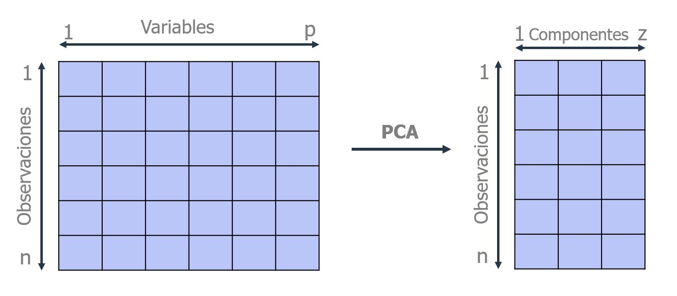
The PCA method therefore allows you to "condense" the information provided by multiple variables into just a few components. However, it is important to remember that you still need the values of the original variables to calculate the components. Two main applications of PCA are visualization and preprocessing of predictors before fitting supervised models.
The scikitlearn library contains the sklearn.decomposition.PCA class, which implements most of the functionalities needed to create and use PCA models. For visualizations, Yellowbrick offers extra features.
Linear Algebra
This section describes two of the mathematical concepts applied in PCA: eigenvectors and eigenvalues. This is simply an intuitive description with the sole purpose of facilitating the understanding of principal component calculation.
Eigenvectors
Eigenvectors are a particular case of multiplication between a matrix and a vector. Consider the following multiplication:
$$\begin{pmatrix} 2 & 3 \\ 2 & 1 \end{pmatrix} x \begin{pmatrix} 3 \\ 2 \end{pmatrix} = \begin{pmatrix} 12 \\ 8 \end{pmatrix} = 4 \ x \begin{pmatrix} 3 \\ 2 \end{pmatrix}$$The resulting vector from the multiplication is an integer multiple of the original vector. The eigenvectors of a matrix are all those vectors that, when multiplied by that matrix, result in the same vector or an integer multiple of it. Eigenvectors have a series of specific mathematical properties:
Eigenvectors only exist for square matrices and not for all of them. If an n x n matrix has eigenvectors, their number is n.
If an eigenvector is scaled before being multiplied by the matrix, the result is a multiple of the same eigenvector. This is because scaling a vector by multiplying it by a certain amount only changes its length but not its direction.
All eigenvectors of a matrix are perpendicular (orthogonal) to each other, regardless of their dimensions.
Given the property that multiplying an eigenvector only changes its length but not its nature as an eigenvector, it is common to scale them so that their length is 1. This way, all of them are standardized. Below is an example:
The eigenvector $\begin{pmatrix} 3 \\ 2 \end{pmatrix}$ has a length of $\sqrt{3^2 + 2^2} = \sqrt{13}$. If each dimension is divided by the length of the vector, the standardized eigenvector with length 1 is obtained.
$$\begin{pmatrix} 3 \\ 2 \end{pmatrix} \div \sqrt{13} = \begin{pmatrix} 3/ \sqrt{13} \\ 2/ \sqrt{13} \end{pmatrix}$$Eigenvalue
When a matrix is multiplied by one of its eigenvectors, the result is a multiple of the original vector, i.e., the result is that same vector multiplied by a number. The value by which the resulting eigenvector is multiplied is known as the eigenvalue. Every eigenvector has a corresponding eigenvalue and vice versa.
In the PCA method, each component corresponds to an eigenvector, and the order of the components is established in decreasing order of eigenvalue. Thus, the first component is the eigenvector with the highest eigenvalue.
Geometric Interpretation of Principal Components
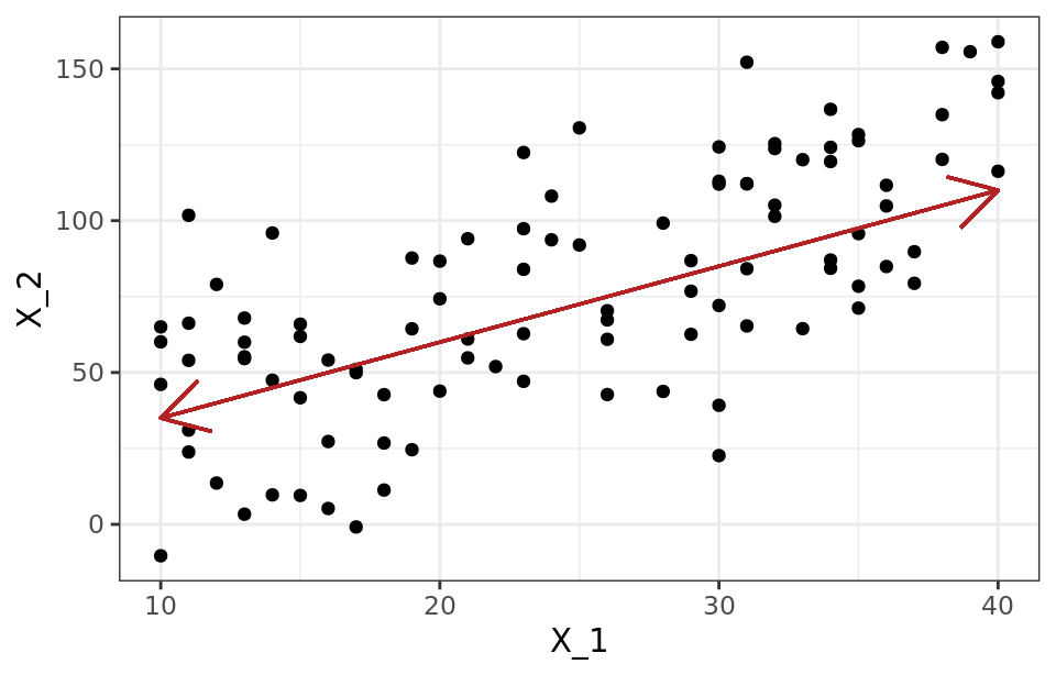
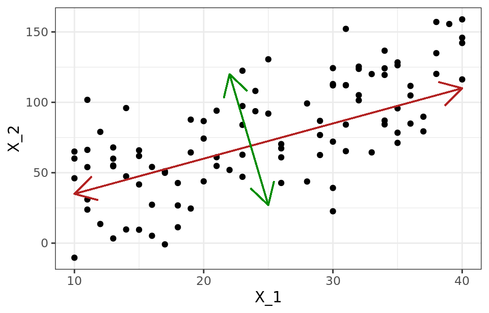
An intuitive way to understand the PCA process is to interpret the principal components from a geometric point of view. Suppose a set of observations for which two variables ($X_1$, $X_2$) are available. The vector that defines the first principal component ($Z_1$) follows the direction in which the observations have the most variance (red line). The projection of each observation onto that direction is equivalent to the value of the first component for that observation (principal component score, $z_{i1}$).
The second component ($Z_2$) follows the second direction in which the data show the greatest variance and is not correlated with the first component. The condition of no correlation between principal components is equivalent to saying that their directions are perpendicular/orthogonal.
Calculation of Principal Components
Each principal component ($Z_i$) is obtained by a linear combination of the original variables. They can be understood as new variables obtained by combining the original variables in a certain way. The first principal component of a group of variables ($X_1$, $X_2$, ..., $X_p$) is the normalized linear combination of those variables that has the greatest variance:
$$Z_1 = \phi_{11} X_1 + \phi_{21}X_2+ ... + \phi_{p1}X_p$$That the linear combination is normalized implies that:
$$\displaystyle\sum_{j=1}^p \phi^{2}_{j1}= 1$$The terms $\phi_{11}$, ..., $\phi_{1p}$ are called loadings and are what define the components. For example, $\phi_{11}$ is the loading of variable $X_1$ for the first principal component. The loadings can be interpreted as the weight/importance that each variable has in each component and, therefore, help to understand what type of information each component captures.
Given a dataset $X$ with n observations and p variables, the process to calculate the first principal component is:
Center the variables: subtract the mean of each variable from its values. This ensures that all variables have zero mean.
Solve an optimization problem to find the value of the loadings that maximize the variance. One way to solve this optimization is by calculating the eigenvector-eigenvalue of the covariance matrix.
Once the first component ($Z_1$) is calculated, the second ($Z_2$) is calculated by repeating the same process but adding the condition that the linear combination cannot be correlated with the first component. This is equivalent to saying that $Z_1$ and $Z_2$ must be perpendicular. The process is repeated iteratively until all possible components (min(n-1, p)) are calculated or until the process is stopped. The order of importance of the components is given by the magnitude of the eigenvalue associated with each eigenvector.
Variable Scaling
The PCA process identifies the directions with the greatest variance. Since the variance of a variable is measured in its own units squared, if all variables are not standardized to have zero mean and unit standard deviation before calculating the components, those variables with a larger scale will dominate the rest. That is why it is always recommended to standardize the data.
Reproducibility of Components
The standard PCA process is deterministic; it always generates the same principal components, i.e., the resulting loadings are the same. The only difference that may occur is that the sign of all the loadings is inverted. This is because the loading vector determines the direction of the component, and that direction is the same regardless of the sign (the component follows a line that extends in both directions). Similarly, the specific value of the components obtained for each observation (principal component scores) is always the same, except for the sign.
Influence of Outliers
Since PCA works with variances, it is very sensitive to outliers, so it is advisable to check for their presence. Detecting outliers with respect to a particular dimension is relatively easy using graphical checks. However, when dealing with multiple dimensions, the process becomes more complicated. For example, consider a man who is 2 meters tall and weighs 50 kg. Neither value is individually an outlier, but together they would be a very exceptional case.
Proportion of Explained Variance
One of the most frequent questions after performing PCA is: How much information present in the original dataset is lost when projecting the observations into a lower-dimensional space? Or, in other words, how much information is each of the obtained principal components able to capture? To answer these questions, we use the proportion of variance explained by each principal component.
Assuming the variables have been normalized to have zero mean, the total variance present in the dataset is defined as
$$\displaystyle\sum_{j=1}^p Var(X_j) = \displaystyle\sum_{j=1}^p \frac{1}{n} \displaystyle\sum_{i=1}^n x^{2}_{ij}$$and the variance explained by component m is
$$\frac{1}{n} \sum_{i=1}^n z^{2}_{im} = \frac{1}{n} \sum_{i=1}^n \left( \sum_{j=1}^p \phi_{jm}x_{ij} \right)^2$$Therefore, the proportion of variance explained by component m is given by the ratio
$$\frac{\sum_{i=1}^n \left( \sum_{j=1}^p \phi_{jm}x_{ij} \right)^2} {\sum_{j=1}^p \sum_{i=1}^n x^{2}_{ij}} $$Both the proportion of explained variance and the proportion of cumulative explained variance are very useful values when deciding the number of principal components to use in subsequent analyses. If all principal components of a dataset are calculated, then, although transformed, all the information present in the original data is retained. The sum of the cumulative explained variance proportion of all components is always 1.
Optimal Number of Principal Components
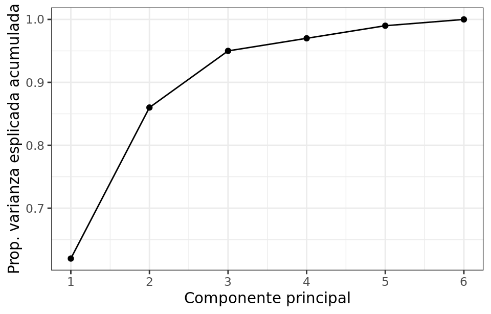
In general, given a data matrix of dimensions n x p, the maximum number of principal components that can be calculated is n-1 or p (the smaller of the two values is the limiting factor). However, since the goal of PCA is to reduce dimensionality, it is usually of interest to use the minimum number of components that are sufficient to explain the data. There is no single answer or method to identify the optimal number of principal components to use. A very common approach is to evaluate the cumulative explained variance proportion and select the minimum number of components after which the increase is no longer substantial.
PCA Example
Libraries
The libraries used in this document are:
# Data processing
# ==============================================================================
import numpy as np
import pandas as pd
import statsmodels.api as sm
# Plots
# ==============================================================================
import matplotlib.pyplot as plt
import matplotlib.font_manager
from matplotlib import style
style.use('ggplot') or plt.style.use('ggplot')
# Preprocessing and modeling
# ==============================================================================
from sklearn.decomposition import PCA
from sklearn.pipeline import make_pipeline
from sklearn.preprocessing import StandardScaler
from sklearn.preprocessing import scale
# Warnings configuration
# ==============================================================================
import warnings
warnings.filterwarnings('ignore')
Data
The USArrests dataset contains the percentage of assaults (Assault), murders (Murder), and rapes (Rape) per 100,000 inhabitants for each of the 50 US states (1973). It also includes the percentage of each state's population living in urban areas (UrbanPoP).
# Data reading
# ==============================================================================
USArrests = sm.datasets.get_rdataset("USArrests", "datasets")
data = USArrests.data
data.head(4)
| Murder | Assault | UrbanPop | Rape | |
|---|---|---|---|---|
| rownames | ||||
| Alabama | 13.2 | 236 | 58 | 21.2 |
| Alaska | 10.0 | 263 | 48 | 44.5 |
| Arizona | 8.1 | 294 | 80 | 31.0 |
| Arkansas | 8.8 | 190 | 50 | 19.5 |
Initial Exploration
The two main aspects to consider when performing PCA are identifying the average value and dispersion of the variables.
The mean of the variables shows that there are three times more rapes than murders and 8 times more assaults than rapes.
print('----------------------')
print('Mean of each variable')
print('----------------------')
data.mean(axis=0)
---------------------- Mean of each variable ----------------------
Murder 7.788 Assault 170.760 UrbanPop 65.540 Rape 21.232 dtype: float64
The variance is very different among the variables; in the case of Assault, the variance is several orders of magnitude higher than the rest.
print('-------------------------')
print('Variance of each variable')
print('-------------------------')
data.var(axis=0)
------------------------- Variance of each variable -------------------------
Murder 18.970465 Assault 6945.165714 UrbanPop 209.518776 Rape 87.729159 dtype: float64
If the variables are not standardized to have zero mean and unit standard deviation before performing the PCA study, the variable Assault, which has a much higher mean and dispersion than the rest, will dominate most of the principal components.
PCA Model
The sklearn.decomposition.PCA class incorporates the main functionalities needed when working with PCA models. The n_components argument determines the number of components calculated. If set to None, all possible components are calculated (min(rows, columns) - 1).
By default, PCA() centers the values but does not scale them. This is important because if the variables have different dispersions, as in this case, they need to be scaled. One way to do this is to combine a StandardScaler() and a PCA() within a pipeline. For more information on using pipelines, see Pipeline and ColumnTransformer.
# Train PCA model with data scaling
# ==============================================================================
pca_pipe = make_pipeline(StandardScaler(), PCA())
pca_pipe.fit(data)
# Extract the trained model from the pipeline
pca_model = pca_pipe.named_steps['pca']
Interpretation
Once the PCA object is trained, you can access all the information about the created components.
components_ contains the value of the loadings $\phi$ that define each component (eigenvector). The rows correspond to the principal components (ordered from highest to lowest explained variance). The columns correspond to the input variables.
# Convert the array to a dataframe to add axis names
# ==============================================================================
pd.DataFrame(
data = pca_model.components_,
columns = data.columns,
index = ['PC1', 'PC2', 'PC3', 'PC4']
)
| Murder | Assault | UrbanPop | Rape | |
|---|---|---|---|---|
| PC1 | 0.535899 | 0.583184 | 0.278191 | 0.543432 |
| PC2 | -0.418181 | -0.187986 | 0.872806 | 0.167319 |
| PC3 | -0.341233 | -0.268148 | -0.378016 | 0.817778 |
| PC4 | -0.649228 | 0.743407 | -0.133878 | -0.089024 |
Analyzing in detail the loading vector that forms each component can help interpret what type of information each one captures. For example, the first component is the result of the following linear combination of the original variables:
$$\text{PC1} = 0.535899 \text{ Murder} + 0.583184 \text{ Assault} + 0.278191 \text{ UrbanPop} + 0.543432 \text{ Rape}$$The weights assigned in the first component to the variables Assault, Murder, and Rape are approximately equal to each other and higher than that assigned to UrbanPoP. This means that the first component mainly captures information related to crimes. In the second component, the variable UrbanPoP has by far the highest weight, so it mainly corresponds to the level of urbanization of the state. While in this example the interpretation of the components is quite clear, this is not always the case, especially as the number of variables increases.
The influence of the variables in each component can be visually analyzed with a heatmap plot.
# Heatmap of components
# ==============================================================================
fig, ax = plt.subplots(nrows=1, ncols=1, figsize=(4, 2))
components = pca_model.components_
plt.imshow(components.T, cmap='viridis', aspect='auto')
plt.yticks(range(len(data.columns)), data.columns)
plt.xticks(range(len(data.columns)), np.arange(pca_model.n_components_) + 1)
plt.grid(False)
plt.colorbar();

Once the principal components are calculated, you can find out the variance explained by each of them, the proportion relative to the total, and the cumulative explained variance proportion. This information is stored in the explained_variance_ and explained_variance_ratio_ attributes of the model.
# Percentage of variance explained by each component
# ==============================================================================
print('----------------------------------------------------')
print('Percentage of variance explained by each component')
print('----------------------------------------------------')
print(pca_model.explained_variance_ratio_)
fig, ax = plt.subplots(nrows=1, ncols=1, figsize=(6, 4))
ax.bar(
x = np.arange(pca_model.n_components_) + 1,
height = pca_model.explained_variance_ratio_
)
for x, y in zip(np.arange(len(data.columns)) + 1, pca_model.explained_variance_ratio_):
label = round(y, 2)
ax.annotate(
label,
(x,y),
textcoords="offset points",
xytext=(0,10),
ha='center'
)
ax.set_xticks(np.arange(pca_model.n_components_) + 1)
ax.set_ylim(0, 1.1)
ax.set_title('Percentage of variance explained by each component')
ax.set_xlabel('Principal component')
ax.set_ylabel('Explained variance (%)');
---------------------------------------------------- Percentage of variance explained by each component ---------------------------------------------------- [0.62006039 0.24744129 0.0891408 0.04335752]

In this case, the first component explains 62% of the variance observed in the data and the second 24.7%. The last two components do not individually exceed 1% of explained variance.
# Cumulative percentage of explained variance
# ==============================================================================
cum_explained_variance = pca_model.explained_variance_ratio_.cumsum()
print('------------------------------------------')
print('Cumulative percentage of explained variance')
print('------------------------------------------')
print(cum_explained_variance)
fig, ax = plt.subplots(nrows=1, ncols=1, figsize=(6, 4))
ax.plot(
np.arange(len(data.columns)) + 1,
cum_explained_variance,
marker = 'o'
)
for x, y in zip(np.arange(len(data.columns)) + 1, cum_explained_variance):
label = round(y, 2)
ax.annotate(
label,
(x,y),
textcoords="offset points",
xytext=(0,10),
ha='center'
)
ax.set_ylim(0, 1.1)
ax.set_xticks(np.arange(pca_model.n_components_) + 1)
ax.set_title('Cumulative percentage of explained variance')
ax.set_xlabel('Principal component')
ax.set_ylabel('Cumulative variance (%)');
------------------------------------------ Cumulative percentage of explained variance ------------------------------------------ [0.62006039 0.86750168 0.95664248 1. ]

If only the first two components were used, 87% of the observed variance would be explained.
Transformation
Once the model is trained, the transform() method can be used to reduce the dimensionality of new observations by projecting them into the space defined by the components.
# Projection of training observations
# ==============================================================================
projections = pca_pipe.transform(X=data)
projections = pd.DataFrame(
projections,
columns = ['PC1', 'PC2', 'PC3', 'PC4'],
index = data.index
)
projections.head()
| PC1 | PC2 | PC3 | PC4 | |
|---|---|---|---|---|
| rownames | ||||
| Alabama | 0.985566 | -1.133392 | -0.444269 | -0.156267 |
| Alaska | 1.950138 | -1.073213 | 2.040003 | 0.438583 |
| Arizona | 1.763164 | 0.745957 | 0.054781 | 0.834653 |
| Arkansas | -0.141420 | -1.119797 | 0.114574 | 0.182811 |
| California | 2.523980 | 1.542934 | 0.598557 | 0.341996 |
The transformation is the result of multiplying the vectors that define each component by the value of the variables. It can be calculated manually:
projections = np.dot(pca_model.components_, scale(data).T)
projections = pd.DataFrame(projections, index = ['PC1', 'PC2', 'PC3', 'PC4'])
projections = projections.transpose().set_index(data.index)
projections.head()
| PC1 | PC2 | PC3 | PC4 | |
|---|---|---|---|---|
| rownames | ||||
| Alabama | 0.985566 | -1.133392 | -0.444269 | -0.156267 |
| Alaska | 1.950138 | -1.073213 | 2.040003 | 0.438583 |
| Arizona | 1.763164 | 0.745957 | 0.054781 | 0.834653 |
| Arkansas | -0.141420 | -1.119797 | 0.114574 | 0.182811 |
| California | 2.523980 | 1.542934 | 0.598557 | 0.341996 |
Reconstruction
The transformation can be reversed and the initial value reconstructed with the inverse_transform() method. It is important to note that the reconstruction will only be complete if all components have been included.
# Reconstruction of the projections
# ==============================================================================
reconstruction = pca_pipe.inverse_transform(X=projections)
reconstruction = pd.DataFrame(
reconstruction,
columns = data.columns,
index = data.index
)
print('------------------')
print('Original values')
print('------------------')
display(reconstruction.head())
print('---------------------')
print('Reconstructed values')
print('---------------------')
display(data.head())
------------------ Original values ------------------
| Murder | Assault | UrbanPop | Rape | |
|---|---|---|---|---|
| rownames | ||||
| Alabama | 13.2 | 236.0 | 58.0 | 21.2 |
| Alaska | 10.0 | 263.0 | 48.0 | 44.5 |
| Arizona | 8.1 | 294.0 | 80.0 | 31.0 |
| Arkansas | 8.8 | 190.0 | 50.0 | 19.5 |
| California | 9.0 | 276.0 | 91.0 | 40.6 |
--------------------- Reconstructed values ---------------------
| Murder | Assault | UrbanPop | Rape | |
|---|---|---|---|---|
| rownames | ||||
| Alabama | 13.2 | 236 | 58 | 21.2 |
| Alaska | 10.0 | 263 | 48 | 44.5 |
| Arizona | 8.1 | 294 | 80 | 31.0 |
| Arkansas | 8.8 | 190 | 50 | 19.5 |
| California | 9.0 | 276 | 91 | 40.6 |
Principal Components Regression Example
The Principal Components Regression (PCR) method consists of fitting a linear regression model by least squares using as predictors the components generated from a Principal Component Analysis (PCA). In this way, with a reduced number of components, most of the variance in the data can be explained.
In observational studies, it is common to have a large number of variables that can be used as predictors; however, this does not necessarily mean that there is a lot of information. If the variables are correlated with each other, the information they provide is redundant and, in addition, the non-collinearity condition required in least squares regression is violated. Since PCA is useful for eliminating redundant information, using principal components as predictors can improve the regression model. It is important to note that, although Principal Components Regression reduces the number of predictors in the model, it cannot be considered a variable selection method since all variables are needed to calculate the components. The optimal number of principal components to use as predictors in PCR can be identified by cross-validation.
Libraries
The libraries used in this example are:
# Data processing
# ==============================================================================
import numpy as np
import pandas as pd
import statsmodels.api as sm
# Plots
# ==============================================================================
import matplotlib.pyplot as plt
import matplotlib.font_manager
from matplotlib import style
style.use('ggplot') or plt.style.use('ggplot')
# Preprocessing and modeling
# ==============================================================================
from sklearn.decomposition import PCA
from sklearn.pipeline import make_pipeline
from sklearn.preprocessing import StandardScaler
from sklearn.model_selection import KFold
from sklearn.model_selection import GridSearchCV
from sklearn.linear_model import LinearRegression
from sklearn.model_selection import train_test_split
from sklearn.metrics import root_mean_squared_error
import multiprocessing
# Warnings configuration
# ==============================================================================
import warnings
warnings.filterwarnings('once')
Data
The quality department of a food company is responsible for measuring the fat content of the meat it sells. This study is carried out using chemical analysis techniques, a process that is relatively costly in terms of time and resources. An alternative that would reduce costs and optimize time is to use a spectrophotometer (an instrument capable of detecting the absorbance of a material at different wavelengths depending on its characteristics) and infer the fat content from its measurements.
Before this new technique can be validated, the company needs to check what margin of error it has compared to chemical analysis. To do this, the absorbance spectrum is measured at 100 wavelengths in 215 meat samples, whose fat content is also obtained by chemical analysis, and a model is trained to predict the fat content from the values given by the spectrophotometer.
The data meatspec.csv used in this example were obtained from the excellent book Linear Models with R, Second Edition.
# Data
# ==============================================================================
data = pd.read_csv('meatspec.csv')
data = data.drop(columns = data.columns[0])
The dataset contains 101 columns. The first 100, named $V1$, ..., $V100$, record the absorbance value for each of the 100 wavelengths analyzed (predictors), and the fat column is the fat content measured by chemical techniques (response variable).
Many of the variables are highly correlated (absolute correlation > 0.8), which is a problem when using linear regression models.
# Correlation between numeric columns
# ==============================================================================
def tidy_corr_matrix(corr_mat):
'''
Function to convert a pandas correlation matrix to tidy format
'''
corr_mat = corr_mat.stack().reset_index()
corr_mat.columns = ['variable_1','variable_2','r']
corr_mat = corr_mat.loc[corr_mat['variable_1'] != corr_mat['variable_2'], :]
corr_mat['abs_r'] = np.abs(corr_mat['r'])
corr_mat = corr_mat.sort_values('abs_r', ascending=False)
return(corr_mat)
corr_matrix = data.select_dtypes(include=['float64', 'int']) \
.corr(method='pearson')
display(tidy_corr_matrix(corr_matrix).head(5))
| variable_1 | variable_2 | r | abs_r | |
|---|---|---|---|---|
| 1019 | V11 | V10 | 0.999996 | 0.999996 |
| 919 | V10 | V11 | 0.999996 | 0.999996 |
| 1121 | V12 | V11 | 0.999996 | 0.999996 |
| 1021 | V11 | V12 | 0.999996 | 0.999996 |
| 917 | V10 | V9 | 0.999996 | 0.999996 |
Models
Two linear models are fitted, one with all predictors and another with only some of the components obtained by PCA, to identify which is better able to predict the fat content of the meat based on the signals recorded by the spectrophotometer.
To evaluate the predictive capacity of each model, the available observations are divided into two groups: one for training (70%) and one for testing (30%).
# Split the data into train and test sets
# ==============================================================================
X = data.drop(columns='fat')
y = data['fat']
X_train, X_test, y_train, y_test = train_test_split(
X,
y,
train_size = 0.7,
random_state = 1234,
shuffle = True
)
Ordinary Least Squares (OLS)
# Model creation and training
# ==============================================================================
modelo = LinearRegression()
modelo.fit(X = X_train, y = y_train)
LinearRegression()In a Jupyter environment, please rerun this cell to show the HTML representation or trust the notebook.
On GitHub, the HTML representation is unable to render, please try loading this page with nbviewer.org.
Parameters
| fit_intercept | True | |
| copy_X | True | |
| tol | 1e-06 | |
| n_jobs | None | |
| positive | False |
# Test predictions
# ==============================================================================
predicciones = modelo.predict(X=X_test)
predicciones = predicciones.flatten()
# Test error of the model
# ==============================================================================
rmse_ols = root_mean_squared_error(
y_true = y_test,
y_pred = predicciones
)
print("")
print(f"The test (rmse) error is: {rmse_ols}")
The test (rmse) error is: 3.839667585624623
The predictions of the final model deviate on average 3.84 units from the actual value.
PCR
To combine PCA with linear regression, a pipeline is created that combines both processes. Since the optimal number of components cannot be known a priori, cross-validation is used.
# Train regression model preceded by PCA with scaling
# ==============================================================================
pipe_model = make_pipeline(StandardScaler(), PCA(), LinearRegression())
pipe_model.fit(X=X_train, y=y_train)
Pipeline(steps=[('standardscaler', StandardScaler()), ('pca', PCA()),
('linearregression', LinearRegression())])In a Jupyter environment, please rerun this cell to show the HTML representation or trust the notebook. On GitHub, the HTML representation is unable to render, please try loading this page with nbviewer.org.
Parameters
| steps | [('standardscaler', ...), ('pca', ...), ...] | |
| transform_input | None | |
| memory | None | |
| verbose | False |
Parameters
| copy | True | |
| with_mean | True | |
| with_std | True |
Parameters
| n_components | None | |
| copy | True | |
| whiten | False | |
| svd_solver | 'auto' | |
| tol | 0.0 | |
| iterated_power | 'auto' | |
| n_oversamples | 10 | |
| power_iteration_normalizer | 'auto' | |
| random_state | None |
Parameters
| fit_intercept | True | |
| copy_X | True | |
| tol | 1e-06 | |
| n_jobs | None | |
| positive | False |
First, the model is evaluated when all components are included.
# Test predictions
# ==============================================================================
predictions = pipe_model.predict(X=X_test)
predictions = predictions.flatten()
# Test error of the model
# ==============================================================================
rmse_pcr = root_mean_squared_error(
y_true = y_test,
y_pred = predictions
)
print("")
print(f"The test (rmse) error is: {rmse_pcr}")
The test (rmse) error is: 3.8396675856416405
# Grid of evaluated hyperparameters
# ==============================================================================
param_grid = {'pca__n_components': [1, 2, 4, 6, 8, 10, 15, 20, 30, 50]}
# Grid search with cross-validation
# ==============================================================================
grid = GridSearchCV(
estimator = pipe_model,
param_grid = param_grid,
scoring = 'neg_root_mean_squared_error',
n_jobs = multiprocessing.cpu_count() - 1,
cv = KFold(n_splits=5),
refit = True,
verbose = 0,
return_train_score = True
)
grid.fit(X = X_train, y = y_train)
# Results
# ==============================================================================
results = pd.DataFrame(grid.cv_results_)
results.filter(regex = '(param.*|mean_t|std_t)') \
.drop(columns = 'params') \
.sort_values('mean_test_score', ascending = False) \
.head(3)
| param_pca__n_components | mean_test_score | std_test_score | mean_train_score | std_train_score | |
|---|---|---|---|---|---|
| 8 | 30 | -2.710551 | 1.104449 | -1.499120 | 0.071778 |
| 5 | 10 | -2.791629 | 0.416056 | -2.448375 | 0.109985 |
| 6 | 15 | -2.842055 | 0.585350 | -2.247184 | 0.099187 |
# Plot cross-validation results for each hyperparameter
# ==============================================================================
fig, ax = plt.subplots(nrows=1, ncols=1, figsize=(7, 3.84), sharey=True)
results.plot('param_pca__n_components', 'mean_train_score', ax=ax)
results.plot('param_pca__n_components', 'mean_test_score', ax=ax)
ax.fill_between(results.param_pca__n_components.astype(float),
results['mean_train_score'] + results['std_train_score'],
results['mean_train_score'] - results['std_train_score'],
alpha=0.2)
ax.fill_between(results.param_pca__n_components.astype(float),
results['mean_test_score'] + results['std_test_score'],
results['mean_test_score'] - results['std_test_score'],
alpha=0.2)
ax.legend()
ax.set_title('CV error evolution')
ax.set_ylabel('neg_root_mean_squared_error');

# Best hyperparameters by cross-validation
# ==============================================================================
print("----------------------------------------")
print("Best hyperparameters found (cv)")
print("----------------------------------------")
print(grid.best_params_, ":", grid.best_score_, grid.scoring)
----------------------------------------
Best hyperparameters found (cv)
----------------------------------------
{'pca__n_components': 30} : -2.7105505991489536 neg_root_mean_squared_error
The cross-validation results show that the best model is obtained using the first 30 components. However, considering the evolution of the error and its interval, after 5 components there are no significant improvements. Following the principle of parsimony, the best model is the one that uses only the first 5 components. The model is retrained with this configuration.
# Train regression model preceded by PCA with scaling
# ==============================================================================
pipe_model = make_pipeline(StandardScaler(), PCA(n_components=5), LinearRegression())
pipe_model.fit(X=X_train, y=y_train)
Pipeline(steps=[('standardscaler', StandardScaler()),
('pca', PCA(n_components=5)),
('linearregression', LinearRegression())])In a Jupyter environment, please rerun this cell to show the HTML representation or trust the notebook. On GitHub, the HTML representation is unable to render, please try loading this page with nbviewer.org.
Parameters
| steps | [('standardscaler', ...), ('pca', ...), ...] | |
| transform_input | None | |
| memory | None | |
| verbose | False |
Parameters
| copy | True | |
| with_mean | True | |
| with_std | True |
Parameters
| n_components | 5 | |
| copy | True | |
| whiten | False | |
| svd_solver | 'auto' | |
| tol | 0.0 | |
| iterated_power | 'auto' | |
| n_oversamples | 10 | |
| power_iteration_normalizer | 'auto' | |
| random_state | None |
Parameters
| fit_intercept | True | |
| copy_X | True | |
| tol | 1e-06 | |
| n_jobs | None | |
| positive | False |
Finally, the model is evaluated with the test data.
# Test predictions
# ==============================================================================
predictions = pipe_model.predict(X=X_test)
predictions = predictions.flatten()
# Test error of the model
# ==============================================================================
rmse_pcr = root_mean_squared_error(
y_true = y_test,
y_pred = predictions
)
print("")
print(f"The test (rmse) error is: {rmse_pcr}")
The test (rmse) error is: 3.359334804522664
Comparison
Using the first five PCA components as predictors instead of the original variables, the root mean squared error is reduced from 3.84 to 3.36.
Session Information
import session_info
session_info.show(html=False)
----- matplotlib 3.10.1 numpy 2.2.6 pandas 2.3.1 session_info v1.0.1 sklearn 1.7.1 statsmodels 0.14.4 ----- IPython 9.1.0 jupyter_client 8.6.3 jupyter_core 5.7.2 jupyterlab 4.4.5 notebook 7.4.5 ----- Python 3.12.9 | packaged by Anaconda, Inc. | (main, Feb 6 2025, 18:56:27) [GCC 11.2.0] Linux-6.14.0-28-generic-x86_64-with-glibc2.39 ----- Session information updated at 2025-08-20 23:54
Bibliography
Introduction to Machine Learning with Python: A Guide for Data Scientists libro
Python Data Science Handbook by Jake VanderPlas libro
Linear Models with R by Julian J.Faraway libro
An Introduction to Statistical Learning: with Applications in R (Springer Texts in Statistics) libro
OpenIntro Statistics: Fourth Edition by David Diez, Mine Çetinkaya-Rundel, Christopher Barr libro
Points of Significance Principal component analysis by Jake Lever, Martin Krzywinski & Naomi Altman
Citation Instructions
How to cite this document?
If you use this document or any part of it, we appreciate your citation. Thank you very much!
Principal Component Analysis (PCA) with Python by Joaquín Amat Rodrigo, available under an Attribution-NonCommercial-ShareAlike 4.0 International (CC BY-NC-SA 4.0 DEED) license at https://cienciadedatos.net/documentos/py19-pca-python-en.html
Did you like the article? Your support is important
Your contribution will help me continue generating free educational content. Thank you very much! 😊


This document created by Joaquín Amat Rodrigo is licensed under an Attribution-NonCommercial-ShareAlike 4.0 International license.
You are allowed to:
-
Share: copy and redistribute the material in any medium or format.
-
Adapt: remix, transform, and build upon the material.
Under the following terms:
-
Attribution: You must give appropriate credit, provide a link to the license, and indicate if changes were made. You may do so in any reasonable manner, but not in any way that suggests the licensor endorses you or your use.
-
NonCommercial: You may not use the material for commercial purposes.
-
ShareAlike: If you remix, transform, or build upon the material, you must distribute your contributions under the same license as the original.