More about machine learning: Machine Learning with Python
- Linear regression
- Logistic regression
- Decision trees
- Random forest
- Gradient boosting
- Machine learning with Python and Scikitlearn
- Neural Networks
- Principal Component Analysis (PCA)
- Clustering with python
- Anomaly detection with PCA
- Face Detection and Recognition
- Introduction to Graphs and Networks
Introduction
Linear regression is a statistical method that aims to model the relationship between a continuous variable and one or more independent variables by fitting a linear equation. It is called simple linear regression when there is only one independent variable and multiple linear regression when there is more than one. Depending on the context, the modeled variable is referred to as the dependent variable or response variable, while the independent variables are known as regressors, predictors, or features.
Throughout this document, the theoretical foundations of linear regression, key practical considerations, and examples of how to create these models in Python are progressively described.
Linear Regression Models in Python
Two of the most commonly used implementations of linear regression models in Python are: scikit-learn and statsmodels. Although both are highly optimized, Scikit-learn is mainly focused on prediction, which means it lacks functionalities to display many of the model characteristics necessary for inference. Statsmodels, on the other hand, is much more comprehensive in this regard.
Mathematical Definition
The linear regression model (Legendre, Gauss, Galton, and Pearson) assumes that, given a set of observations
$\{y_i, x_{i1},...,x_{ip}\}^{n}_{i=1}$, the mean $\mu$ of the response variable $y$ is linearly related to the regressors $x_1, ..., x_p$ according to the equation:
The result of this equation is known as the population regression line, which captures the relationship between the predictors and the mean of the response variable.
Another common definition found in statistical literature is:
$$ y_i = \beta_0 + \beta_1 x_{i1} + \beta_2 x_{i2} + ... + \beta_p x_{ip} + \epsilon_i $$In this case, the equation refers to the value of $y$ for a specific observation $i$. Since an individual observation will never be exactly equal to the mean, an error term $\epsilon$ is included.
In both cases, the interpretation of the model components is the same:
$\beta_0$: The intercept, representing the average value of the response variable $y$ when all predictors are zero.
$\beta_j$: The partial regression coefficient, representing the average effect on $y$ when predictor $x_j$ increases by one unit, keeping the other variables constant.
$\epsilon$: The residual (error term), representing the difference between the observed and estimated values of $y$. It captures the influence of all factors affecting $y$ that are not included in the model.
In most cases, the population values $\beta_0$ and $\beta_j$ are unknown. Therefore, their estimates $\hat{\beta}_0$ and $\hat{\beta}_j$ are obtained from a sample. Fitting the model consists of estimating the regression coefficients from the available data in a way that maximizes the likelihood, meaning it identifies the model most likely to have generated the observed data.
The most commonly used method for this estimation is Ordinary Least Squares (OLS), which finds the best-fitting line (or plane, in the case of multiple regression) by minimizing the sum of squared vertical deviations between each training data point and the regression line.
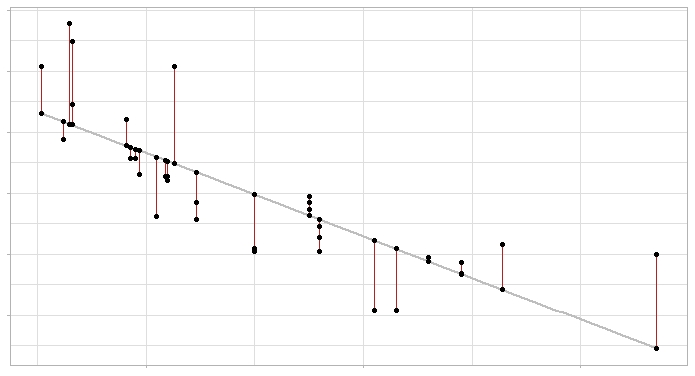
Linear regression model and its errors: the gray line represents the regression line (the model) and the red segments show the error between the line and each observation.
Computationally, these calculations are more efficient when performed in matrix form:
$$ \mathbf{y} = \mathbf{X}^T \mathbf{\beta} + \epsilon $$Once the coefficients are estimated, the estimates for each observation ($\hat{y}_i$) can be obtained as:
$$ \hat{y}_i = \hat{\beta}_0 + \hat{\beta}_1 x_{i1} + \hat{\beta}_2 x_{i2} + \dots + \hat{\beta}_p x_{ip} $$Finally, the estimate of the model's variance ($\hat{\sigma}^2$) is obtained as:
$$ \hat{\sigma}^2 = \frac{\sum^n_{i=1} \hat{\epsilon}_i^2}{n-p} = \frac{\sum^n_{i=1} (y_i - \hat{y}_i)^2}{n-p} $$where $n$ is the number of observations and $p$ is the number of predictors.
Model interpretation
The main elements to interpret in a linear regression model are the predictor coefficients:
$\beta_{0}$ is the intercept, which corresponds to the expected value of the response variable $y$ when all predictors are zero.
$\beta_{j}$, the partial regression coefficients of each predictor, indicate the expected average change in the response variable $y$ when the predictor variable $x_{j}$ increases by one unit, while keeping the other variables constant.
The magnitude of each partial regression coefficient depends on the units in which the corresponding predictor variable is measured, so its magnitude is not associated with the importance of each predictor.
To determine the impact of each variable in the model, standardized partial coefficients are used. These are obtained by standardizing (subtracting the mean and dividing by the standard deviation) the predictor variables before fitting the model. In this case, $\beta_{0}$ corresponds to the expected value of the response variable when all predictors are at their mean value, and $\beta_{j}$ represents the expected average change in the response variable when the predictor variable $x_{j}$ increases by one standard deviation, keeping the other variables constant.
While regression coefficients are usually the primary focus when interpreting a linear model, there are many other aspects to consider (overall model significance, predictor significance, normality condition, etc.). These aspects are often given little attention when the sole objective of the model is to make predictions. However, they become highly relevant when performing inference, that is, explaining the relationships between predictors and the response variable. Each of these aspects will be introduced throughout this document.
Meaning of "Linear"
The term "linear" in regression models refers to the fact that the parameters are incorporated into the equation in a linear manner, not necessarily that the relationship between each predictor and the response variable must follow a linear pattern.
The following equation shows a linear model in which the predictor $x_1$ is not linearly related to y:
$$y = \beta_0 + \beta_1x_1 + \beta_2log(x_1) + \epsilon$$import numpy as np
import matplotlib.pyplot as plt
plt.style.use('fivethirtyeight')
plt.rcParams.update({'font.size': 10, 'lines.linewidth': 1.5})
x1 = np.linspace(1,5, num=100)
x2 = np.linspace(1,5, num=100)
y = 0.0 + 0.5*x1 - 0.8*np.log(x2)
fig, ax = plt.subplots(figsize=(5, 2.5))
ax.plot(x1, y)
ax.set_xlabel("x1")
ax.set_ylabel("y");

In contrast, the following equation does not represent a linear model:
$$y = \beta_0 + \beta_1x_1^{\beta_2} + \epsilon$$However, some nonlinear relationships can be transformed into a linear form:
$$y = \beta_0x_1^{\beta_1}\epsilon $$Taking the logarithm on both sides:
$$\log(y) = \log(\beta_0) + \beta_1 \log(x_1) + \log(\epsilon)$$This transformation allows the model to be expressed in a linear form, making it suitable for linear regression techniques.
Goodness of Fit of the Model
Once the model has been fitted, it is necessary to verify its usefulness, as even though it represents the best-fitting line among all possible ones, it may still have a large error. The most commonly used metrics to assess the quality of fit are the Residual Standard Error (RSE) and the Coefficient of Determination ($R^2$).
Residual Standard Error (RSE)
The Residual Standard Error (RSE) measures the average deviation of any estimated point from the regression line. It has the same units as the response variable. A common way to determine whether the RSE is high is by dividing it by the mean value of the response variable, thereby obtaining a percentage deviation.
$$RSE = \sqrt{\frac{1}{n-p-1}RSS}$$In simple linear regression models, since there is only one predictor, $(n-p-1) = (n-2)$.
Coefficient of Determination ($R^2$)
$R^2$ describes the proportion of variance in the response variable explained by the model relative to the total variance. Its value ranges between 0 and 1. Since it is dimensionless, it has the advantage of being easier to interpret compared to RSE.
$$R^{2}=\frac{\text{Total Sum of Squares - Residual Sum of Squares}}{\text{Total Sum of Squares}}=$$ $$1-\frac{\text{Residual Sum of Squares}}{\text{Total Sum of Squares}} = $$ $$1-\frac{\sum(\hat{y_i}-y_i)^2}{\sum(y_i-\overline{y})^2}$$In simple linear regression models, the $R^2$ value corresponds to the square of the Pearson correlation coefficient (r) between $x$ and $y$. However, this is not the case in multiple regression.
In multiple linear regression models, the more predictors included in the model, the higher the $R^2$ value. This happens because each predictor, even if only slightly, helps explain part of the variability observed in $y$. For this reason, $R^2$ cannot be used to compare models with different numbers of predictors.
$R^2_{adjusted}$ introduces a penalty to the $R^2$ value for each predictor added to the model. The value of the penalty depends on the number of predictors used and the sample size, i.e., the degrees of freedom. The larger the sample size, the more predictors can be included in the model. Adjusted $R^2$ helps find the best model, the one that explains the variability in $y$ most effectively with the fewest predictors.
$$R^{2}_{adj} = 1 - \frac{SSE}{SST} \times \frac{n-1}{n-p-1} = R^{2} - (1-R^{2}) \frac{n-1}{n-p-1} = 1 - \frac{SSE/df_{e}}{SST/df_{t}}$$where $SSE$ is the variability explained by the model (Sum of Squares Explained), $SST$ is the total variability of $y$ (Sum of Squares Total), $n$ is the sample size, and $p$ is the number of predictors included in the model.
Model Significance F-test
One of the first results to evaluate when fitting a linear model is the outcome of the $F$-test. This test answers the question of whether the model as a whole can predict the response variable better than expected by chance, or equivalently, if at least one of the predictors in the model contributes significantly. To perform this test, the sum of squared residuals of the model of interest is compared to that of the model without predictors, which consists only of the mean (also known as the total sum of squares, $TSS$).
$$F = \frac{(TSS - RSS)/(p-1)}{RSS/(n-p)}$$Frequently, the null and alternative hypotheses for this test are described as:
- $H_0$: $\beta_1$ = ... = $\beta_{p-1} = 0$
- $H_a$: at least one $\beta_i \neq 0$
If the $F$ test is significant, it implies that the model is useful, but it does not necessarily mean it is the best model. It could happen that one of its predictors is unnecessary.
Significance of the Predictors
In most cases, although regression analysis is applied to a sample, the ultimate goal is to obtain a linear model that explains the relationship between the variables in the entire population. This means that the generated model is an estimate of the population relationship based on the relationship observed in the sample and, therefore, is subject to variations. For each of the coefficients in the linear regression equation ($\beta_j$), its significance (p-value) and confidence interval can be calculated. The most commonly used statistical test is the $T$-test$, although there are non-parametric alternatives.
The significance test for the coefficients ($\beta_j$) in the linear model considers the following hypotheses:
$H_0$: the predictor $x_j$ does not contribute to the model ($\beta_j = 0$), in the presence of the other predictors. In the case of simple linear regression, it can also be interpreted as there being no linear relationship between the two variables, meaning the slope of the model is zero $\beta_j = 0$.
$H_a$: the predictor $x_j$ does contribute to the model ($\beta_j \neq 0$), in the presence of the other predictors. In the case of simple linear regression, it can also be interpreted as there being a linear relationship between the two variables, meaning the slope of the model is not zero $\beta_j \neq 0$.
Calculation of the T-statistic and the p-value:
where
$$SE(\hat{\beta}_j)^2 = \frac{\sigma^2}{\sum^n_{i=1}(x_{ji} -\overline{x})^2}$$The error variance $\sigma^2$ is estimated from the Residual Standard Error (RSE), which can be understood as the average difference by which the response variable deviates from the true regression line. In the case of simple linear regression, RSE is equivalent to:
$$RSE = \sqrt{\frac{1}{n-2}RSS} = \sqrt{\frac{1}{n-2}\sum^n_{i=1}(y_i -\hat{y}_i)}$$Degrees of freedom (df) = number of observations - 2 = number of observations - number of predictors - 1
p-value = P(|t| > calculated t value)
Confidence Intervals
The fewer the number of observations $n$, the less capacity there is to calculate the model's standard error. As a consequence, the accuracy of the estimated regression coefficients decreases. This is especially important in multiple regression.
In models generated with statsmodels, along with the regression coefficient values, the t-statistic value for each is returned, along with the p-values and corresponding confidence intervals. This allows to know, in addition to the estimates, whether they are significantly different from 0, i.e., if they contribute to the model.
For the calculations described above to be valid, it must be assumed that the residuals are independent and that they are normally distributed with a mean of 0 and variance $\sigma^2$. When the normality condition is not met, there is the possibility of using permutation tests to calculate significance (p-value) and bootstrapping to calculate confidence intervals.
Categorical Variables as Predictors
When a categorical variable is introduced as a predictor, one level is taken as the reference level (usually coded as 0) against which the other levels are compared. If the categorical predictor has more than two levels, so-called dummy variables or one-hot encoding are generated. These are variables created for each level of the categorical predictor that can take the value of 0 or 1. Each time the model is used to predict a value, only one dummy variable per predictor takes the value of 1 (the one corresponding to the level the predictor takes in that case), while the rest are considered 0. The partial regression coefficient $\beta_j$ for each dummy variable indicates the average percentage influence of that level on the dependent variable $y$ in comparison to the reference level of that predictor.
The concept of dummy variables is better understood with an example. Suppose a model in which the response variable weight is predicted based on height and nationality of the subject. The nationality variable is qualitative with 3 levels (American, European, and Asian). Even though the initial predictor is nationality, a new variable is created for each level, which can be either 0 or 1. Thus, the equation of the complete model is:
$$weight = \beta_0 + \beta_1height + \beta_2american + \beta_3european + \beta_4asian$$If the subject is European, the dummy variables for American and Asian are considered 0, so the model for this case is:
$$weight = \beta_0 + \beta_1height + \beta_3european$$Prediction
Once a valid model has been generated, it is possible to predict the value of the response variable $y$ for new values of the predictor variables $x$. It is important to note that predictions should a priori be restricted to the range of values within which the observations used to train the model fall. This is important because, although linear models can be extrapolated, it is only within this range that we are confident that the conditions for the model to be valid are met. The equation generated by the regression is used to calculate the predictions:
$$\hat{y}_i= \hat{\beta}_0 + \hat{\beta}_1 x_{i1} + \hat{\beta}_2 x_{i2} + ... + \hat{\beta}_p x_{ip}$$Since the model is obtained from a sample, the estimates of the regression coefficients have an associated error, and so do the predicted values generated from them. There are two ways of measuring the uncertainty associated with a prediction:
- Confidence intervals: the interval for the average expected value of the response variable $y$ for a given value of $x$.
- Prediction intervals: the interval for the expected value of the response variable $y$ for a given value of $x$.
Although both seem similar, the difference lies in the fact that confidence intervals are applied to the average expected value of $y$ for a given value of $x$, whereas prediction intervals are not applied to the average. For this reason, the latter are always wider than the former.
A characteristic that stems from how the margin of error is calculated in both confidence and prediction intervals is that the interval widens as the values of $x$ approach the extremes of the observed range.
import seaborn as sns
import pandas as pd
import matplotlib.pyplot as plt
bateos = [5659, 5710, 5563, 5672, 5532, 5600, 5518, 5447, 5544, 5598,
5585, 5436, 5549, 5612, 5513, 5579, 5502, 5509, 5421, 5559,
5487, 5508, 5421, 5452, 5436, 5528, 5441, 5486, 5417, 5421]
runs = [855, 875, 787, 730, 762, 718, 867, 721, 735, 615, 708, 644, 654, 735,
667, 713, 654, 704, 731, 743, 619, 625, 610, 645, 707, 641, 624, 570,
593, 556]
data = pd.DataFrame({'hits': bateos, 'runs': runs})
fig, ax = plt.subplots(figsize=(5, 2.5))
sns.regplot(x='runs', y='hits', data=data, ax = ax);

Why does this happen? By paying attention to the equation for the standard error of the confidence interval, the numerator contains the term $(x_k - \bar{x})^2$ (the same happens for the prediction interval).
$$\sqrt{MSE \left(\frac{1}{n} + \frac{(x_k - \bar{x})^2}{\sum^n_{i=1}(x_i - \bar{x}^2)} \right)}$$This term corresponds to the squared difference between the value $x_k$ for which the prediction is being made and the mean $\bar{x}$ of the observed values of the predictor $x$. The further $x_k$ is from $\bar{x}$, the larger the numerator becomes, and therefore the larger the standard error. This is why the intervals widen as the values of $x$ move away from the mean of the observed values.
Model Validation
Once the best model that can be created with the available data is selected, its ability to predict new observations that were not used for training must be verified. This way, it can be checked if the model can generalize. A commonly used strategy is to randomly split the data into two groups, fit the model with the first group, and estimate the prediction accuracy using the second.
The appropriate size of the partitions largely depends on the amount of available data and the level of confidence needed in the error estimation. An 80%-20% split generally yields good results.
A more robust strategy is to use cross-validation, which consists of dividing the data into $k$ groups (folds) and using $k-1$ of them to train the model and the remaining one to estimate the prediction error. This process is repeated $k$ times, each time using a different fold as the test set. The final error is the average of the errors obtained in each iteration.
Conditions for Linear Regression
For a linear regression model using least squares, and the conclusions drawn from it, to be completely valid, the assumptions underlying its mathematical development must be verified. In practice, it is rare that all assumptions are met or can be proven to be met. However, this does not mean the model is not useful. What is important is to be aware of these assumptions and the impact they may have on the conclusions drawn from the model.
No Collinearity or Multicollinearity:
In multiple linear models, the predictors must be independent; there should be no collinearity between them. Collinearity occurs when a predictor is linearly related to one or more of the other predictors in the model. As a result of collinearity, the individual effect of each predictor on the response variable cannot be accurately identified, which leads to an increase in the variance of the estimated regression coefficients to the point where it becomes impossible to establish their statistical significance. Additionally, small changes in the data cause large changes in the coefficient estimates. While true collinearity only exists when the simple or multiple correlation coefficient between predictors is 1, which rarely happens in reality, it is common to encounter what is known as near-collinearity or imperfect multicollinearity.
There is no specific statistical method to determine the existence of collinearity or multicollinearity between the predictors of a regression model. However, many practical rules have been developed to assess the impact on the model. The recommended steps are:
If the coefficient of determination $R^2$ is high, but none of the predictors are significant, there are indications of collinearity.
Create a correlation matrix that calculates the linear relationship between each pair of predictors. It is important to note that even if no high correlation coefficients are obtained, multicollinearity cannot be ruled out. There may be a nearly perfect linear relationship between three or more variables, and the simple correlations between pairs of these variables may not exceed 0.5.
Generate a simple linear regression model for each predictor against the others. If any of these models has a high coefficient of determination $R^2$, it may indicate potential collinearity.
Tolerance (TOL) and Variance Inflation Factor (VIF). These are two parameters that essentially quantify the same thing (one is the inverse of the other). The VIF of each predictor is calculated using the following formula:
Where $R^2$ is obtained from the regression of predictor $X_j$ on the other predictors. This is the most recommended approach, and the reference limits commonly used are:
VIF = 1: complete absence of collinearity.
1 < VIF < 5: the regression may be affected by some collinearity.
5 < VIF < 10: the regression may be highly affected by some collinearity.
The tolerance term is $\frac{1}{VIF}$, so the recommended limits are between 1 and 0.1.
If collinearity between predictors is found, there are two possible solutions. The first is to exclude one of the problematic predictors while attempting to retain the one that, in the researcher's judgment, is truly influencing the response variable. This measure generally has little impact on the model's predictive capacity, as, in the presence of collinearity, the information provided by one predictor is redundant in the presence of the other. The second option is to combine the collinear variables into a single predictor, though this carries the risk of losing its interpretation.
When trying to establish cause-and-effect relationships, collinearity can lead to very erroneous conclusions, making it seem that one variable is the cause when, in reality, another is influencing that predictor.
Linear Relationship Between Numeric Predictors and the Response Variable
Each numeric predictor must be linearly related to the response variable $y$, while keeping the other predictors constant. If this condition is not met, the predictor should not be included in the model. The most recommended way to check this is by plotting the residuals of the model against each of the predictors. If the relationship is linear, the residuals will be randomly distributed around zero. These analyses are only approximate, as it is not possible to definitively determine if the relationship is truly linear while keeping the other predictors constant.
Normal Distribution of the Response Variable
The response variable must follow a normal distribution. To verify this, histograms, normal quantile plots, or hypothesis tests for normality are commonly used.
Constant Variance of the Response Variable (Homoscedasticity)
The variance of the response variable must remain constant across the range of predictors. To verify this, it is common to plot the model's residuals against each predictor. If the variance is constant, the residuals will scatter randomly with consistent dispersion and no specific pattern. A conical distribution is a clear sign of a lack of homoscedasticity. Homoscedasticity tests, such as the Breusch-Pagan test, can also be used.
The reason for this condition is as follows: linear models assume that the response variable ($y$) follows a normal distribution, with a mean ($\mu$) that can be modeled as a function of other variables (predictors), and whose variance ($\sigma$) is calculated using a dispersion constant and a function $\nu(\mu)$. This means that the variance is not directly modeled as a function of the predictors, but indirectly through its relationship with the mean, and it is a unique value.
$$\hat{\sigma}^2 = \frac{\sum^n_{i=1} \hat{\epsilon}_i^2}{n-p} = \frac{\sum^n_{i=1} (y_i - \hat{\mu})^2}{n-p}$$What impact can this have in practice? While the estimates of the mean obtained by these models are good, the uncertainties associated with them, and consequently the confidence and prediction intervals that can be calculated, may not be as accurate.
No Autocorrelation (Independence)
The values of each observation must be independent of the others. It is recommended to plot the residuals in the order of the time at which the observations were recorded. If any pattern is present, this may indicate autocorrelation. The Durbin-Watson hypothesis test can also be used to check for autocorrelation.
Outliers, High Leverage, or Influential Points
It is important to identify observations that are outliers or may be influencing the model. The easiest way to detect them is through the residuals (more details to follow).
Sample Size
This is not a condition in itself, but if there are not enough observations, predictors that are not truly influential might appear to be. A common recommendation is that the number of observations should be at least 10 to 20 times the number of predictors in the model.
Parsimony (Occam's razor)
This term refers to the idea that the best model is the one that can explain the observed variability in the response variable with the fewest predictors, and therefore, with fewer assumptions.
The vast majority of conditions are verified using the residuals, so the model is typically generated first, and then the conditions are validated. In fact, fitting a model should be seen as an iterative process where the model is adjusted, its residuals are evaluated, and improvements are made. This continues until an optimal model is reached.
Outliers
Regardless of whether the model is accepted, it is always advisable to identify any potential outliers, high leverage observations, or influential points, as they could significantly influence the model. The decision to remove such observations should be carefully considered, depending on the purpose of the model. If the goal is predictive, a model without outliers or highly influential observations is usually better at predicting most cases. However, it is very important to pay attention to these values because, if they are not measurement errors, they could represent the most interesting cases. The proper course of action when suspecting an outlier or influential point is to fit the regression model both including and excluding the value in question.
Example of Simple Linear Regression
Suppose a sports analyst wants to know if there is a relationship between the number of times a baseball team’s players hit and the number of runs they score. If such a relationship exists and a model can be established, this model could be used to predict the outcome of a game.
Libraries
Libraries used in this example are:
# Data management
# ==============================================================================
import pandas as pd
# Plots
# ==============================================================================
import matplotlib.pyplot as plt
# Preprocessing and modeling
# ==============================================================================
from scipy.stats import pearsonr
from sklearn.linear_model import LinearRegression
from sklearn.model_selection import train_test_split
from sklearn.metrics import root_mean_squared_error
import statsmodels.api as sm
# Matplotlib settings
# ==============================================================================
plt.style.use('fivethirtyeight')
plt.rcParams.update({'font.size': 10, 'lines.linewidth': 1.5})
# Warnings
# ==============================================================================
import warnings
warnings.filterwarnings('once')
Data
# Data
# ==============================================================================
teams = ["Texas","Boston","Detroit","Kansas","St.","New_S.","New_Y.",
"Milwaukee","Colorado","Houston","Baltimore","Los_An.","Chicago",
"Cincinnati","Los_P.","Philadelphia","Chicago","Cleveland","Arizona",
"Toronto","Minnesota","Florida","Pittsburgh","Oakland","Tampa",
"Atlanta","Washington","San.F","San.I","Seattle"]
hits = [5659, 5710, 5563, 5672, 5532, 5600, 5518, 5447, 5544, 5598,
5585, 5436, 5549, 5612, 5513, 5579, 5502, 5509, 5421, 5559,
5487, 5508, 5421, 5452, 5436, 5528, 5441, 5486, 5417, 5421]
runs = [855, 875, 787, 730, 762, 718, 867, 721, 735, 615, 708, 644, 654, 735,
667, 713, 654, 704, 731, 743, 619, 625, 610, 645, 707, 641, 624, 570,
593, 556]
data = pd.DataFrame({'team': teams, 'hits': hits, 'runs': runs})
data.head(3)
| team | hits | runs | |
|---|---|---|---|
| 0 | Texas | 5659 | 855 |
| 1 | Boston | 5710 | 875 |
| 2 | Detroit | 5563 | 787 |
Exploratory Data Analysis
The first step before generating a simple regression model is to visualize the data to intuitively assess if a relationship exists and quantify this relationship using a correlation coefficient.
# Plot
# ==============================================================================
fig, ax = plt.subplots(figsize=(4, 3))
data.plot(
x = 'hits',
y = 'runs',
c = 'firebrick',
kind = "scatter",
ax = ax
)
ax.set_title('Distribution of hits and runs');

# Linear correlation between the two variables
# ==============================================================================
corr_test = pearsonr(x=data["hits"], y=data["runs"])
print(f"Correlation coefficient: {corr_test[0]}")
print(f"P-value: {corr_test[1]}")
Correlation coefficient: 0.6106270467206688 P-value: 0.00033883513597919785
The graph and the correlation test show a linear relationship, with considerable strength (r = 0.61) and significance (p-value = 0.000339). It makes sense to attempt generating a linear regression model with the goal of predicting the number of runs based on the team's number of hits.
Model Fitting
A model is fitted using runs as the response variable and hits as the predictor. As in any predictive study, it is not only important to fit the model but also to quantify its ability to predict new observations. To evaluate this, the data is split into two groups: a training set and a test set.
Scikit-learn
# Data partition into training and test set
# ==============================================================================
X = data[['hits']]
y = data['runs']
X_train, X_test, y_train, y_test = train_test_split(
X,
y,
train_size = 0.8,
random_state = 1234,
shuffle = True
)
# Create and fit the model
# ==============================================================================
model = LinearRegression()
model.fit(X=X_train, y=y_train)
LinearRegression()In a Jupyter environment, please rerun this cell to show the HTML representation or trust the notebook.
On GitHub, the HTML representation is unable to render, please try loading this page with nbviewer.org.
LinearRegression()
# Information about the model
# ==============================================================================
print(f"Intercept: {model.intercept_}")
print(f"Coeficient: {list(zip(model.feature_names_in_, model.coef_))}")
print(f"Coefficient of determination R^2: {model.score(X, y)}")
Intercept: -2367.702841302211
Coeficient: [('hits', 0.5528713534479736)]
Coefficient of determination R^2: 0.3586119899498744
Once the model is trained, its predictive ability is evaluated using the test set.
# Prediction error (rmse) on the test set
# ==============================================================================
predictions = model.predict(X=X_test)
rmse = root_mean_squared_error(y_true=y_test, y_pred=predictions)
print(f"First five predicctions: {predictions[0:5]}")
print(f"Error (rmse) on the test set: {rmse}")
First five predicctions: [643.78742093 720.0836677 690.78148597 789.19258689 627.20128033] Error (rmse) on the test set: 59.336716083360486
Statsmodels
The Statsmodels linear regression implementation is more complete than that of Scikit-learn, as it not only fits the model but also allows the calculation of statistical tests and necessary analyses to verify that the conditions upon which this type of model is based are met. Statsmodels has two ways to train the model:
Indicating the model formula and passing the training data as a dataframe that includes the response variable and predictors. This method is similar to the one used in R.
Passing two matrices, one for the predictors and another for the response variable. This is the same as the one used by Scikit-learn, with the difference that the predictors matrix must include an additional column of 1s.
# Data partition into training and test set
# ==============================================================================
X = data[['hits']]
y = data['runs']
X_train, X_test, y_train, y_test = train_test_split(
X,
y,
train_size = 0.8,
random_state = 1234,
shuffle = True
)
# Create and fit the model
# ==============================================================================
# A column of 1s is added at the beginning of the matrix for the intercept
X_train = sm.add_constant(X_train, prepend=True)
model = sm.OLS(endog=y_train, exog=X_train)
model = model.fit()
print(model.summary())
OLS Regression Results
==============================================================================
Dep. Variable: runs R-squared: 0.271
Model: OLS Adj. R-squared: 0.238
Method: Least Squares F-statistic: 8.191
Date: Thu, 13 Feb 2025 Prob (F-statistic): 0.00906
Time: 18:03:13 Log-Likelihood: -134.71
No. Observations: 24 AIC: 273.4
Df Residuals: 22 BIC: 275.8
Df Model: 1
Covariance Type: nonrobust
==============================================================================
coef std err t P>|t| [0.025 0.975]
------------------------------------------------------------------------------
const -2367.7028 1066.357 -2.220 0.037 -4579.192 -156.214
hits 0.5529 0.193 2.862 0.009 0.152 0.953
==============================================================================
Omnibus: 5.033 Durbin-Watson: 1.902
Prob(Omnibus): 0.081 Jarque-Bera (JB): 3.170
Skew: 0.829 Prob(JB): 0.205
Kurtosis: 3.650 Cond. No. 4.17e+05
==============================================================================
Notes:
[1] Standard Errors assume that the covariance matrix of the errors is correctly specified.
[2] The condition number is large, 4.17e+05. This might indicate that there are
strong multicollinearity or other numerical problems.
Confidence Intervals of the Coefficients
# Confidence intervals for model coefficients
# ==============================================================================
intervals = model.conf_int(alpha=0.05)
intervals.columns = ['2.5%', '97.5%']
intervals
| 2.5% | 97.5% | |
|---|---|---|
| const | -4579.192050 | -156.213633 |
| hits | 0.152244 | 0.953499 |
Predicctions
Once the model is trained, predictions can be obtained for new data. The Statsmodels models allow you to calculate predictions in two ways:
.predict(): returns only the prediction values..get_prediction().summary_frame(): returns the predictions along with the associated confidence intervals.
# Predictions with 95% confidence interval
# ==============================================================================
predicctions = model.get_prediction(exog=X_train).summary_frame(alpha=0.05)
predicctions.head(4)
| mean | mean_se | mean_ci_lower | mean_ci_upper | obs_ci_lower | obs_ci_upper | |
|---|---|---|---|---|---|---|
| 3 | 768.183475 | 32.658268 | 700.454374 | 835.912577 | 609.456054 | 926.910897 |
| 23 | 646.551778 | 19.237651 | 606.655332 | 686.448224 | 497.558860 | 795.544695 |
| 14 | 680.276930 | 14.186441 | 650.856053 | 709.697807 | 533.741095 | 826.812765 |
| 13 | 735.011194 | 22.767596 | 687.794091 | 782.228298 | 583.893300 | 886.129088 |
Graphical Representation of the Model
In addition to the least squares line, it is advisable to include the upper and lower bounds of the confidence interval. This helps identify the region where, according to the generated model and for a given confidence level, the average value of the response variable is expected to lie.
# Predictions with 95% confidence interval
# ==============================================================================
predicctions = model.get_prediction(exog=X_train).summary_frame(alpha=0.05)
predicctions['x'] = X_train.loc[:, 'hits']
predicctions['y'] = y_train
predicctions = predicctions.sort_values('x')
# Plot
# ==============================================================================
fig, ax = plt.subplots(figsize=(6, 3.84))
ax.scatter(predicctions['x'], predicctions['y'], marker='o', color = "gray")
ax.plot(predicctions['x'], predicctions["mean"], linestyle='-', label="OLS")
ax.plot(predicctions['x'], predicctions["mean_ci_lower"], linestyle='--', color='blue', label="95% CI")
ax.plot(predicctions['x'], predicctions["mean_ci_upper"], linestyle='--', color='blue')
ax.fill_between(predicctions['x'], predicctions["mean_ci_lower"], predicctions["mean_ci_upper"], alpha=0.3)
ax.legend();

Test error
# Error on the test set
# ==============================================================================
X_test = sm.add_constant(X_test, prepend=True)
predictions = model.predict(exog=X_test)
rmse = root_mean_squared_error(y_true=y_test, y_pred=predictions)
print(f"The error (rmse) on the test set is: {rmse}")
The error (rmse) on the test set is: 59.33671608336119
Interpretation
print(model.summary())
OLS Regression Results
==============================================================================
Dep. Variable: runs R-squared: 0.271
Model: OLS Adj. R-squared: 0.238
Method: Least Squares F-statistic: 8.191
Date: Thu, 13 Feb 2025 Prob (F-statistic): 0.00906
Time: 18:03:14 Log-Likelihood: -134.71
No. Observations: 24 AIC: 273.4
Df Residuals: 22 BIC: 275.8
Df Model: 1
Covariance Type: nonrobust
==============================================================================
coef std err t P>|t| [0.025 0.975]
------------------------------------------------------------------------------
const -2367.7028 1066.357 -2.220 0.037 -4579.192 -156.214
hits 0.5529 0.193 2.862 0.009 0.152 0.953
==============================================================================
Omnibus: 5.033 Durbin-Watson: 1.902
Prob(Omnibus): 0.081 Jarque-Bera (JB): 3.170
Skew: 0.829 Prob(JB): 0.205
Kurtosis: 3.650 Cond. No. 4.17e+05
==============================================================================
Notes:
[1] Standard Errors assume that the covariance matrix of the errors is correctly specified.
[2] The condition number is large, 4.17e+05. This might indicate that there are
strong multicollinearity or other numerical problems.
The column (coef) returns the estimated value for the two parameters of the linear model equation ($\hat{\beta}_0$ and $\hat{\beta}_1$), which correspond to the intercept (intercept or const) and the slope.
The standard errors, the t-statistic value, and the two-tailed p-value for each of the two parameters are also shown. This allows us to determine whether the predictors are significantly different from 0, meaning they have importance in the model. For the generated model, both the intercept and the slope are significant (p-values < 0.05).
The R-squared value indicates that the model can explain 27.1% of the observed variability in the response variable (runs). Additionally, the p-value obtained in the F-test (Prob (F-statistic) = 0.00906) suggests that there is evidence that the variance explained by the model is greater than what would be expected by chance (total variance).
The generated linear model follows the equation:
$$\text{runs = -2367.7028 + 0.5529 hits}$$For each unit increase in the number of hits, the number of runs increases on average by 0.5529 units.
The test error of the model is 59.34. The predictions of the final model deviate on average by 59.34 units from the actual value.
Multiple Linear Regression Example
Suppose the sales department of a company wants to study the influence of advertising through different channels on the number of product sales. A dataset is available containing the revenue (in millions) obtained from sales in 200 regions, as well as the budget allocated (also in millions) for advertisements on radio, TV, and newspapers in each region.
Libraríes
The libraries used in this example are:
# Tratamiento de data
# ==============================================================================
import pandas as pd
import numpy as np
# Gráficos
# ==============================================================================
import matplotlib.pyplot as plt
import seaborn as sns
# Preprocesado y modelado
# ==============================================================================
from scipy.stats import pearsonr
from sklearn.model_selection import train_test_split
from sklearn.metrics import root_mean_squared_error
import statsmodels.api as sm
import statsmodels.formula.api as smf
from statsmodels.stats.anova import anova_lm
from scipy import stats
# Configuración matplotlib
# ==============================================================================
plt.style.use('fivethirtyeight')
plt.rcParams.update({'font.size': 10, 'lines.linewidth': 1.5})
# Configuración warnings
# ==============================================================================
import warnings
warnings.filterwarnings('ignore')
Data
# Data
# ==============================================================================
tv = [230.1, 44.5, 17.2, 151.5, 180.8, 8.7, 57.5, 120.2, 8.6, 199.8, 66.1, 214.7,
23.8, 97.5, 204.1, 195.4, 67.8, 281.4, 69.2, 147.3, 218.4, 237.4, 13.2,
228.3, 62.3, 262.9, 142.9, 240.1, 248.8, 70.6, 292.9, 112.9, 97.2, 265.6,
95.7, 290.7, 266.9, 74.7, 43.1, 228.0, 202.5, 177.0, 293.6, 206.9, 25.1,
175.1, 89.7, 239.9, 227.2, 66.9, 199.8, 100.4, 216.4, 182.6, 262.7, 198.9,
7.3, 136.2, 210.8, 210.7, 53.5, 261.3, 239.3, 102.7, 131.1, 69.0, 31.5,
139.3, 237.4, 216.8, 199.1, 109.8, 26.8, 129.4, 213.4, 16.9, 27.5, 120.5,
5.4, 116.0, 76.4, 239.8, 75.3, 68.4, 213.5, 193.2, 76.3, 110.7, 88.3, 109.8,
134.3, 28.6, 217.7, 250.9, 107.4, 163.3, 197.6, 184.9, 289.7, 135.2, 222.4,
296.4, 280.2, 187.9, 238.2, 137.9, 25.0, 90.4, 13.1, 255.4, 225.8, 241.7, 175.7,
209.6, 78.2, 75.1, 139.2, 76.4, 125.7, 19.4, 141.3, 18.8, 224.0, 123.1, 229.5,
87.2, 7.8, 80.2, 220.3, 59.6, 0.7, 265.2, 8.4, 219.8, 36.9, 48.3, 25.6, 273.7,
43.0, 184.9, 73.4, 193.7, 220.5, 104.6, 96.2, 140.3, 240.1, 243.2, 38.0, 44.7,
280.7, 121.0, 197.6, 171.3, 187.8, 4.1, 93.9, 149.8, 11.7, 131.7, 172.5, 85.7,
188.4, 163.5, 117.2, 234.5, 17.9, 206.8, 215.4, 284.3, 50.0, 164.5, 19.6, 168.4,
222.4, 276.9, 248.4, 170.2, 276.7, 165.6, 156.6, 218.5, 56.2, 287.6, 253.8, 205.0,
139.5, 191.1, 286.0, 18.7, 39.5, 75.5, 17.2, 166.8, 149.7, 38.2, 94.2, 177.0,
283.6, 232.1]
radio = [37.8, 39.3, 45.9, 41.3, 10.8, 48.9, 32.8, 19.6, 2.1, 2.6, 5.8, 24.0, 35.1,
7.6, 32.9, 47.7, 36.6, 39.6, 20.5, 23.9, 27.7, 5.1, 15.9, 16.9, 12.6, 3.5,
29.3, 16.7, 27.1, 16.0, 28.3, 17.4, 1.5, 20.0, 1.4, 4.1, 43.8, 49.4, 26.7,
37.7, 22.3, 33.4, 27.7, 8.4, 25.7, 22.5, 9.9, 41.5, 15.8, 11.7, 3.1, 9.6,
41.7, 46.2, 28.8, 49.4, 28.1, 19.2, 49.6, 29.5, 2.0, 42.7, 15.5, 29.6, 42.8,
9.3, 24.6, 14.5, 27.5, 43.9, 30.6, 14.3, 33.0, 5.7, 24.6, 43.7, 1.6, 28.5,
29.9, 7.7, 26.7, 4.1, 20.3, 44.5, 43.0, 18.4, 27.5, 40.6, 25.5, 47.8, 4.9,
1.5, 33.5, 36.5, 14.0, 31.6, 3.5, 21.0, 42.3, 41.7, 4.3, 36.3, 10.1, 17.2,
34.3, 46.4, 11.0, 0.3, 0.4, 26.9, 8.2, 38.0, 15.4, 20.6, 46.8, 35.0, 14.3,
0.8, 36.9, 16.0, 26.8, 21.7, 2.4, 34.6, 32.3, 11.8, 38.9, 0.0, 49.0, 12.0,
39.6, 2.9, 27.2, 33.5, 38.6, 47.0, 39.0, 28.9, 25.9, 43.9, 17.0, 35.4, 33.2,
5.7, 14.8, 1.9, 7.3, 49.0, 40.3, 25.8, 13.9, 8.4, 23.3, 39.7, 21.1, 11.6, 43.5,
1.3, 36.9, 18.4, 18.1, 35.8, 18.1, 36.8, 14.7, 3.4, 37.6, 5.2, 23.6, 10.6, 11.6,
20.9, 20.1, 7.1, 3.4, 48.9, 30.2, 7.8, 2.3, 10.0, 2.6, 5.4, 5.7, 43.0, 21.3, 45.1,
2.1, 28.7, 13.9, 12.1, 41.1, 10.8, 4.1, 42.0, 35.6, 3.7, 4.9, 9.3, 42.0, 8.6]
newspaper = [69.2, 45.1, 69.3, 58.5, 58.4, 75.0, 23.5, 11.6, 1.0, 21.2, 24.2, 4.0,
65.9, 7.2, 46.0, 52.9, 114.0, 55.8, 18.3, 19.1, 53.4, 23.5, 49.6, 26.2,
18.3, 19.5, 12.6, 22.9, 22.9, 40.8, 43.2, 38.6, 30.0, 0.3, 7.4, 8.5, 5.0,
45.7, 35.1, 32.0, 31.6, 38.7, 1.8, 26.4, 43.3, 31.5, 35.7, 18.5, 49.9,
36.8, 34.6, 3.6, 39.6, 58.7, 15.9, 60.0, 41.4, 16.6, 37.7, 9.3, 21.4, 54.7,
27.3, 8.4, 28.9, 0.9, 2.2, 10.2, 11.0, 27.2, 38.7, 31.7, 19.3, 31.3, 13.1,
89.4, 20.7, 14.2, 9.4, 23.1, 22.3, 36.9, 32.5, 35.6, 33.8, 65.7, 16.0, 63.2,
73.4, 51.4, 9.3, 33.0, 59.0, 72.3, 10.9, 52.9, 5.9, 22.0, 51.2, 45.9, 49.8,
100.9, 21.4, 17.9, 5.3, 59.0, 29.7, 23.2, 25.6, 5.5, 56.5, 23.2, 2.4, 10.7,
34.5, 52.7, 25.6, 14.8, 79.2, 22.3, 46.2, 50.4, 15.6, 12.4, 74.2, 25.9, 50.6,
9.2, 3.2, 43.1, 8.7, 43.0, 2.1, 45.1, 65.6, 8.5, 9.3, 59.7, 20.5, 1.7, 12.9,
75.6, 37.9, 34.4, 38.9, 9.0, 8.7, 44.3, 11.9, 20.6, 37.0, 48.7, 14.2, 37.7,
9.5, 5.7, 50.5, 24.3, 45.2, 34.6, 30.7, 49.3, 25.6, 7.4, 5.4, 84.8, 21.6, 19.4,
57.6, 6.4, 18.4, 47.4, 17.0, 12.8, 13.1, 41.8, 20.3, 35.2, 23.7, 17.6, 8.3,
27.4, 29.7, 71.8, 30.0, 19.6, 26.6, 18.2, 3.7, 23.4, 5.8, 6.0, 31.6, 3.6, 6.0,
13.8, 8.1, 6.4, 66.2, 8.7]
sells = [22.1, 10.4, 9.3, 18.5, 12.9, 7.2, 11.8, 13.2, 4.8, 10.6, 8.6, 17.4, 9.2, 9.7,
19.0, 22.4, 12.5, 24.4, 11.3, 14.6, 18.0, 12.5, 5.6, 15.5, 9.7, 12.0, 15.0, 15.9,
18.9, 10.5, 21.4, 11.9, 9.6, 17.4, 9.5, 12.8, 25.4, 14.7, 10.1, 21.5, 16.6, 17.1,
20.7, 12.9, 8.5, 14.9, 10.6, 23.2, 14.8, 9.7, 11.4, 10.7, 22.6, 21.2, 20.2, 23.7,
5.5, 13.2, 23.8, 18.4, 8.1, 24.2, 15.7, 14.0, 18.0, 9.3, 9.5, 13.4, 18.9, 22.3,
18.3, 12.4, 8.8, 11.0, 17.0, 8.7, 6.9, 14.2, 5.3, 11.0, 11.8, 12.3, 11.3, 13.6,
21.7, 15.2, 12.0, 16.0, 12.9, 16.7, 11.2, 7.3, 19.4, 22.2, 11.5, 16.9, 11.7, 15.5,
25.4, 17.2, 11.7, 23.8, 14.8, 14.7, 20.7, 19.2, 7.2, 8.7, 5.3, 19.8, 13.4, 21.8,
14.1, 15.9, 14.6, 12.6, 12.2, 9.4, 15.9, 6.6, 15.5, 7.0, 11.6, 15.2, 19.7, 10.6,
6.6, 8.8, 24.7, 9.7, 1.6, 12.7, 5.7, 19.6, 10.8, 11.6, 9.5, 20.8, 9.6, 20.7, 10.9,
19.2, 20.1, 10.4, 11.4, 10.3, 13.2, 25.4, 10.9, 10.1, 16.1, 11.6, 16.6, 19.0, 15.6,
3.2, 15.3, 10.1, 7.3, 12.9, 14.4, 13.3, 14.9, 18.0, 11.9, 11.9, 8.0, 12.2, 17.1,
15.0, 8.4, 14.5, 7.6, 11.7, 11.5, 27.0, 20.2, 11.7, 11.8, 12.6, 10.5, 12.2, 8.7,
26.2, 17.6, 22.6, 10.3, 17.3, 15.9, 6.7, 10.8, 9.9, 5.9, 19.6, 17.3, 7.6, 9.7, 12.8,
25.5, 13.4]
data = pd.DataFrame({'tv': tv, 'radio': radio, 'newspaper': newspaper, 'sells': sells})
Relationship Between Variables
The first step in establishing a multiple linear model is to study the relationship between variables. This information is critical for identifying the best predictors for the model and detecting collinearity among predictors. Additionally, it is recommended to visualize the distribution of each variable.
# Correlation between numerical columns
# ==============================================================================
def tidy_corr_matrix(corr_mat):
'''
Fuction to convert a pandas correlation matrix into tidy format
'''
corr_mat = corr_mat.stack().reset_index()
corr_mat.columns = ['variable_1', 'variable_2','r']
corr_mat = corr_mat.loc[corr_mat['variable_1'] != corr_mat['variable_2'], :]
corr_mat['abs_r'] = np.abs(corr_mat['r'])
corr_mat = corr_mat.sort_values('abs_r', ascending=False)
return corr_mat
corr_matrix = data.select_dtypes(include=['float64', 'int']).corr(method='pearson')
tidy_corr_matrix(corr_matrix).head(10)
| variable_1 | variable_2 | r | abs_r | |
|---|---|---|---|---|
| 3 | tv | sells | 0.782224 | 0.782224 |
| 12 | sells | tv | 0.782224 | 0.782224 |
| 7 | radio | sells | 0.576223 | 0.576223 |
| 13 | sells | radio | 0.576223 | 0.576223 |
| 6 | radio | newspaper | 0.354104 | 0.354104 |
| 9 | newspaper | radio | 0.354104 | 0.354104 |
| 11 | newspaper | sells | 0.228299 | 0.228299 |
| 14 | sells | newspaper | 0.228299 | 0.228299 |
| 2 | tv | newspaper | 0.056648 | 0.056648 |
| 8 | newspaper | tv | 0.056648 | 0.056648 |
# Heatmap of the correlation matrix
# ==============================================================================
fig, ax = plt.subplots(nrows=1, ncols=1, figsize=(4, 4))
sns.heatmap(
corr_matrix,
annot = True,
cbar = False,
annot_kws = {"size": 8},
vmin = -1,
vmax = 1,
center = 0,
cmap = sns.diverging_palette(20, 220, n=200),
square = True,
ax = ax
)
ax.set_xticklabels(
ax.get_xticklabels(),
rotation = 45,
horizontalalignment = 'right',
)
ax.tick_params(labelsize = 10)

# Distribution of numerical variables
# ==============================================================================
fig, axes = plt.subplots(nrows=2, ncols=2, figsize=(7, 4))
axes = axes.flat
numeric_cols = data.select_dtypes(include=['float64', 'int']).columns
for i, colum in enumerate(numeric_cols):
sns.histplot(
data = data,
x = colum,
stat = "count",
kde = True,
color = (list(plt.rcParams['axes.prop_cycle']) * 2)[i]["color"],
line_kws= {'linewidth': 2},
alpha = 0.3,
ax = axes[i]
)
axes[i].set_title(colum, fontsize = 8, fontweight = "bold")
axes[i].tick_params(labelsize = 8)
axes[i].set_xlabel("")
axes[i].set_ylabel("")
fig.tight_layout()
plt.subplots_adjust(top = 0.9)
fig.suptitle('Distribution of numerical variables', fontsize = 10, fontweight = "bold");

Model Fitting
A multiple linear model is fitted with the goal of predicting sales based on the investment in the three advertising channels.
# Data partition
# ==============================================================================
X = data[['tv', 'radio', 'newspaper']]
y = data['sells']
X_train, X_test, y_train, y_test = train_test_split(
X,
y,
train_size = 0.8,
random_state = 1234,
shuffle = True
)
# Create and fit the model
# ==============================================================================
# A column of 1s is added at the beginning of the matrix for the intercept
X_train = sm.add_constant(X_train, prepend=True)
model = sm.OLS(endog=y_train, exog=X_train,)
model = model.fit()
print(model.summary())
OLS Regression Results
==============================================================================
Dep. Variable: sells R-squared: 0.894
Model: OLS Adj. R-squared: 0.892
Method: Least Squares F-statistic: 437.8
Date: Thu, 13 Feb 2025 Prob (F-statistic): 1.01e-75
Time: 18:03:15 Log-Likelihood: -308.29
No. Observations: 160 AIC: 624.6
Df Residuals: 156 BIC: 636.9
Df Model: 3
Covariance Type: nonrobust
==============================================================================
coef std err t P>|t| [0.025 0.975]
------------------------------------------------------------------------------
const 2.8497 0.365 7.803 0.000 2.128 3.571
tv 0.0456 0.002 28.648 0.000 0.042 0.049
radio 0.1893 0.009 20.024 0.000 0.171 0.208
newspaper 0.0024 0.007 0.355 0.723 -0.011 0.016
==============================================================================
Omnibus: 53.472 Durbin-Watson: 2.153
Prob(Omnibus): 0.000 Jarque-Bera (JB): 147.411
Skew: -1.353 Prob(JB): 9.77e-33
Kurtosis: 6.846 Cond. No. 472.
==============================================================================
Notes:
[1] Standard Errors assume that the covariance matrix of the errors is correctly specified.
The model with all variables introduced as predictors has a high $R^2$ (0.894), meaning it is able to explain 89.4% of the observed variability in sales. The p-value of the model is significant (1.01e-75), so we can accept that the model is better than expected by chance, and at least one of the partial regression coefficients is different from 0.
According to the p-value obtained for the partial regression coefficient of newspaper (0.723), this variable does not contribute significantly to the model in the presence of the other predictors. The model is retrained, but this time excluding the predictor newspaper.
# Remove the newspaper column from the train and test set
# ==============================================================================
X_train = X_train.drop(columns = 'newspaper')
X_test = X_test.drop(columns = 'newspaper')
X_train = sm.add_constant(X_train, prepend=True)
model = sm.OLS(endog=y_train, exog=X_train,)
model = model.fit()
print(model.summary())
OLS Regression Results
==============================================================================
Dep. Variable: sells R-squared: 0.894
Model: OLS Adj. R-squared: 0.892
Method: Least Squares F-statistic: 660.3
Date: Thu, 13 Feb 2025 Prob (F-statistic): 3.69e-77
Time: 18:03:15 Log-Likelihood: -308.36
No. Observations: 160 AIC: 622.7
Df Residuals: 157 BIC: 631.9
Df Model: 2
Covariance Type: nonrobust
==============================================================================
coef std err t P>|t| [0.025 0.975]
------------------------------------------------------------------------------
const 2.9004 0.335 8.652 0.000 2.238 3.563
tv 0.0456 0.002 28.751 0.000 0.042 0.049
radio 0.1904 0.009 21.435 0.000 0.173 0.208
==============================================================================
Omnibus: 54.901 Durbin-Watson: 2.157
Prob(Omnibus): 0.000 Jarque-Bera (JB): 156.962
Skew: -1.375 Prob(JB): 8.24e-35
Kurtosis: 6.998 Cond. No. 429.
==============================================================================
Notes:
[1] Standard Errors assume that the covariance matrix of the errors is correctly specified.
Confidence Intervals of the Coefficients
# Confidence intervals for model coefficients
# ==============================================================================
intervals = model.conf_int(alpha=0.05)
intervals.columns = ['2.5%', '97.5%']
intervals
| 2.5% | 97.5% | |
|---|---|---|
| const | 2.238211 | 3.562549 |
| tv | 0.042439 | 0.048701 |
| radio | 0.172853 | 0.207942 |
Diagnostic of the reesiduals
# Diagnostic of errors (residues) of training predictions
# ==============================================================================
predictions_train = model.predict(exog=X_train)
residuos_train = predictions_train - y_train
Inspección visual
# Gráficos
# ==============================================================================
fig, axes = plt.subplots(nrows=3, ncols=2, figsize=(8, 8))
axes[0, 0].scatter(y_train, predictions_train, edgecolors=(0, 0, 0), alpha = 0.4)
axes[0, 0].plot([y_train.min(), y_train.max()], [y_train.min(), y_train.max()], 'k--', color = 'black', lw=2)
axes[0, 0].set_title('Prediction vs real value', fontsize = 10, fontweight = "bold")
axes[0, 0].set_xlabel('Real')
axes[0, 0].set_ylabel('Prediction')
axes[0, 0].tick_params(labelsize = 7)
axes[0, 1].scatter(list(range(len(y_train))), residuos_train, edgecolors=(0, 0, 0), alpha = 0.4)
axes[0, 1].axhline(y = 0, linestyle = '--', color = 'black', lw=2)
axes[0, 1].set_title('Residuals', fontsize = 10, fontweight = "bold")
axes[0, 1].set_xlabel('id')
axes[0, 1].set_ylabel('Residual')
axes[0, 1].tick_params(labelsize = 7)
sns.histplot(
data = residuos_train,
stat = "density",
kde = True,
line_kws= {'linewidth': 1},
alpha = 0.3,
ax = axes[1, 0]
)
axes[1, 0].set_title('Distribution of residuals', fontsize = 10, fontweight = "bold")
axes[1, 0].set_xlabel("Residual")
axes[1, 0].tick_params(labelsize = 7)
sm.qqplot(
residuos_train,
fit = True,
line = 'q',
ax = axes[1, 1],
alpha = 0.4,
lw = 2
)
axes[1, 1].set_title('Q-Q residuals', fontsize = 10, fontweight = "bold")
axes[1, 1].tick_params(labelsize = 7)
axes[2, 0].scatter(predictions_train, residuos_train, edgecolors=(0, 0, 0), alpha = 0.4)
axes[2, 0].axhline(y = 0, linestyle = '--', color = 'black', lw=2)
axes[2, 0].set_title('Residuals vs prediction', fontsize = 10, fontweight = "bold")
axes[2, 0].set_xlabel('Prediction')
axes[2, 0].set_ylabel('Residual')
axes[2, 0].tick_params(labelsize = 7)
# Remove empty plot
fig.delaxes(axes[2, 1])
fig.tight_layout()
plt.subplots_adjust(top=0.9)
fig.suptitle('Residual analysis', fontsize = 12, fontweight = "bold");

The residuals do not appear to be randomly distributed around zero, and the variability does not seem to remain consistent across the X-axis. This pattern suggests a lack of homoscedasticity and normal distribution.
Normality Test
The residuals are checked to see if they follow a normal distribution using two statistical tests: the Shapiro-Wilk test and D'Agostino's K-squared test. The latter is included in the statsmodels summary under the name Omnibus.
In both tests, the null hypothesis assumes that the data follows a normal distribution. Therefore, if the p-value is not lower than the selected significance level alpha, there is no evidence to reject the assumption that the data follows a normal distribution.
# Shapiro-Wilk test
# ==============================================================================
shapiro_test = stats.shapiro(residuos_train)
shapiro_test
ShapiroResult(statistic=0.9165122842956668, pvalue=5.861065888990398e-08)
# D'Agostino's K-squared test
# ==============================================================================
k2, p_value = stats.normaltest(residuos_train)
print(f"Estadítico= {k2}, p-value = {p_value}")
Estadítico= 54.90105653039115, p-value = 1.197807558003796e-12
Both tests provide strong evidence to reject the hypothesis that the data follows a normal distribution (p-value << 0.01).
Predictions
Once the model is trained, predictions can be made for new data. Statsmodels models allow for the calculation of confidence intervals associated with each prediction.
# Predictions with 95% confidence interval
# ==============================================================================
predictions = model.get_prediction(exog=X_train).summary_frame(alpha=0.05)
predictions.head(4)
| mean | mean_se | mean_ci_lower | mean_ci_upper | obs_ci_lower | obs_ci_upper | |
|---|---|---|---|---|---|---|
| 146 | 15.231643 | 0.248325 | 14.741154 | 15.722132 | 11.880621 | 18.582665 |
| 32 | 7.615382 | 0.247198 | 7.127119 | 8.103645 | 4.264685 | 10.966079 |
| 43 | 13.928155 | 0.213535 | 13.506384 | 14.349927 | 10.586500 | 17.269810 |
| 99 | 17.001020 | 0.210052 | 16.586127 | 17.415913 | 13.660226 | 20.341814 |
Error on the test set
# Test error
# ==============================================================================
X_test = sm.add_constant(X_test, prepend=True)
predictions = model.predict(exog = X_test)
rmse = root_mean_squared_error(y_true=y_test, y_pred=predictions)
print(f"The error (rmse) on the test set is: {rmse}")
The error (rmse) on the test set is: 1.6956207500101192
Interpretation
The multiple linear regression model:
$$\text{sells = 2.9004 + 0.0456tv + 0.1904radio}$$is able to explain 89.4% of the observed variance in sales (R-squared: 0.894, Adj. R-squared: 0.892). The $F$ test is significant (p-value: 3.69e-77), providing clear evidence that the model explains the variance in sales better than expected by chance. The statistical tests for each variable confirm that tv and radio are related to the number of sales and contribute to the model.
The normality conditions are not satisfied, so the confidence intervals estimated for the coefficients and the predictions are not reliable.
The test error (rmse) is 1.696. The predictions of the final model deviate, on average, by 1.696 units from the actual value.
Interaction Between Predictors
The linear model from which the conclusions have been drawn assumes that the effect on sales due to an increase in the budget of one of the media channels is independent of the budget spent on the others. For example, the linear model considers that the average effect on sales from increasing the TV ad budget by one unit is always 0.0456, regardless of the amount spent on radio ads. However, this does not necessarily have to be the case—there may be interaction between predictors such that the effect of each predictor on the response variable depends, to some extent, on the value of the other predictor.
As previously defined, a linear model with two predictors follows the equation:
$$y=\beta_{0}+\beta_{1}x_{1}+\beta_{2}x_{2}+\epsilon$$According to this definition, an increase of one unit in predictor $x_1$ results in an average increase of the response variable y by $\beta_{1}$. Modifications to predictor $x_2$ do not alter this, and the same applies to $x_2$ with respect to $x_1$. In order for the model to account for the interaction between both, a third predictor, called the interaction term, is introduced, which is the product of predictors $x_1$ and $x_2$.
$$y=\beta_{0}+\beta_{1}x_{1}+\beta_{2}x_{2}+\beta_{3}x_{1}x_{2} + e$$Reorganizing the terms gives:
$$y=\beta_{0}+(\beta_{1} + \beta_{3}x_2)x_{1}+\beta_{2}x_{2}+ e$$Now, the effect of $x_{1}$ on $y$ is no longer constant but depends on the value of $x_{2}$.
In multiple linear regression models that incorporate interactions between predictors, the hierarchical principle must be taken into account. This principle states that if an interaction between predictors is included in the model, the individual predictors involved in the interaction must always be included, regardless of whether their p-value is significant or not.
In statsmodels, interaction between predictors can be introduced in two ways:
By specifying it in the formula with the
*term:sells ~ tv * radioBy adding a new column with the multiplication of the predictors whose interaction is to be included in the model.
# Split data
# ==============================================================================
X = data[['tv', 'radio']]
y = data['sells']
X_train, X_test, y_train, y_test = train_test_split(
X,
y,
train_size = 0.8,
random_state = 1234,
shuffle = True
)
# Creación del model con interacciones utilizando matrices
# ==============================================================================
# Se añade una nueva columna con la interacción
X_train['tv_radio'] = X_train['tv'] * X_train['radio']
X_test['tv_radio'] = X_test['tv'] * X_test['radio']
X_train = sm.add_constant(X_train, prepend=True)
model_interactions = sm.OLS(endog=y_train, exog=X_train,)
model_interactions = model_interactions.fit()
print(model_interactions.summary())
OLS Regression Results
==============================================================================
Dep. Variable: sells R-squared: 0.968
Model: OLS Adj. R-squared: 0.967
Method: Least Squares F-statistic: 1562.
Date: Thu, 13 Feb 2025 Prob (F-statistic): 4.28e-116
Time: 18:03:17 Log-Likelihood: -212.91
No. Observations: 160 AIC: 433.8
Df Residuals: 156 BIC: 446.1
Df Model: 3
Covariance Type: nonrobust
==============================================================================
coef std err t P>|t| [0.025 0.975]
------------------------------------------------------------------------------
const 6.9035 0.281 24.558 0.000 6.348 7.459
tv 0.0183 0.002 10.812 0.000 0.015 0.022
radio 0.0261 0.010 2.623 0.010 0.006 0.046
tv_radio 0.0011 5.86e-05 18.931 0.000 0.001 0.001
==============================================================================
Omnibus: 121.946 Durbin-Watson: 1.686
Prob(Omnibus): 0.000 Jarque-Bera (JB): 1473.094
Skew: -2.642 Prob(JB): 0.00
Kurtosis: 16.894 Cond. No. 1.84e+04
==============================================================================
Notes:
[1] Standard Errors assume that the covariance matrix of the errors is correctly specified.
[2] The condition number is large, 1.84e+04. This might indicate that there are
strong multicollinearity or other numerical problems.
The results show clear evidence that the interaction tv radio is significant (p-value* very close to 0).
The model that incorporates the interaction has an Adjusted R-squared of 0.967, a value higher than the 0.892 of the model that only considered the individual effect of the predictors. However, is this difference enough to claim that the model with interaction is superior? One way to answer this question is by using the F-test (ANOVA).
Comparison of Models Using F-test (ANOVA)
Consider a model $M$ and another smaller model $m$, formed by a subset of the predictors contained in $M$. If the difference in fit is very small, according to the principle of parsimony, model $m$ is more appropriate. It is possible to test if the difference in fit is significant by comparing the residuals. Specifically, the statistic used is:
$$\frac{RSS_m - RSS_M}{RSS_M}$$To avoid the model size influencing the test, the residual sum of squares RSS of each model is divided by its degrees of freedom. The resulting statistic follows an $F$ distribution:
$$\frac{(RSS_m - RSS_M)/(df_m - df_M)}{RSS_M/(df_M)} \sim F_{df_m-df_M, \ df_M}$$where $df$ are the degrees of freedom of the model, which correspond to the number of observations minus the number of predictors.
In the previous sections, a model that included interactions and one that did not were trained. A hypothesis test is now performed to evaluate the null hypothesis that both models fit the data equally well. In other words, to determine whether one model is better than the other in predicting the response variable. This can be done using the anova_lm() function from statsmodels.stats.anova.
anova_lm(model, model_interactions)
| df_resid | ssr | df_diff | ss_diff | F | Pr(>F) | |
|---|---|---|---|---|---|---|
| 0 | 157.0 | 442.212726 | 0.0 | NaN | NaN | NaN |
| 1 | 156.0 | 134.116584 | 1.0 | 308.096142 | 358.3673 | 2.926598e-42 |
The ANOVA test provides clear evidence (p-value virtually zero) that the model including the interaction between predictors is able to model the response variable better.
This method of comparing models is well established in the statistical community. In the machine learning community, it is much more common to compare models using validation techniques such as cross-validation.
Miscellaneous Notes
In this section, I gather comments, definitions, and clarifications I have found in different sources and that I have considered better to keep as supplementary information.
Origin of the Least Squares Method and Regression
Linear Models with R, by Julian J. Faraway
The least squares method was published in 1805 by Adrien Marie Legendre. The term regression comes from a publication by Francis Galton in 1885 called Regression to Mediocrity. In it, Galton used the least squares method to demonstrate that children of tall parents tend to be tall as well, but not as much as their parents, and that children of shorter parents tend to be short, but not as much as their parents.
Estimation of the Variance of a Linear Model by Least Squares
Linear Models with R, by Julian J. Faraway
The estimation of the variance ($\sigma^2$) of a linear model obtained by least squares is:
$$\sigma^2 = \frac{RSS}{n - p}$$The term Residual Standard Error (RSE) is the square root of $\sigma^2$:
$$RSE = \sqrt{\frac{RSS}{n - p}}$$Advantages of the Least Squares Method for Estimating the Coefficients of a Linear Model
Linear Models with R, by Julian J. Faraway
Although there are alternatives to the least squares method for estimating the correlation coefficients $\hat{\beta}_j$ of a linear model, it offers several advantages:
It has a geometric interpretation, which makes it easier to understand.
If the errors are independent and normally distributed, its solution is equivalent to the maximum likelihood estimation.
The $\hat{\beta}_j$ are unbiased estimations.
Identifiability or Collinearity
Linear Models with R, by Julian J. Faraway
The least squares method has a unique solution only if the matrix formed by the predictors has full rank, meaning all its columns (predictors) are linearly independent. In practice, this identifiability condition is often violated. The following are some scenarios where this occurs:
When one of the predictors introduced in the model is a linear transformation or combination of other predictors already in the model. For example, if the variable weight is introduced in both kilograms and pounds, or if predictors like the number of years of basic education, number of years of university education, and total years of education are included. This problem can be avoided by studying the nature of the available variables and their relationships.
Model oversaturation, when there are more predictors than observations.
Caution When Evaluating Residual Normality Through Hypothesis Testing
Linear Models with R, by Julian J. Faraway
For the residuals of a linear regression model to be normally distributed is a necessary condition for the significance (p-value) and the confidence intervals associated with the predictors (calculated from theoretical models) to be accurate. This condition is often evaluated with hypothesis tests such as the Shapiro-Wilk test. When this happens, it is important to understand the relationship between p-value and sample size. With more residuals, the test has greater power, so small deviations from normality become significant. Additionally, the central limit theorem suggests that, as the sample size increases, the results become more robust to deviations from normality. Given these properties, it is usually more advisable to assess the normality of the residuals graphically, using a theoretical quantile-quantile (qq-plot) plot.
Transformation of Variables
Linear Models with R, by Julian J. Faraway and Wikipedia
Transforming the response variable or the predictors can be a way to improve the fit of a model or correct violations of certain regression assumptions.
When the transformation is applied to the response variable, it is important to remember that the predictions generated by the model are on the transformed scale. Once the prediction is made, it can be transformed back to the original scale. The same applies to confidence intervals: first, the upper and lower limits are calculated, and then they are transformed back. In contrast, the regression coefficients obtained for the predictors must be interpreted in the context of the transformation. It is not possible to apply the inverse of the transformation and interpret them on the original scale.
Box-Cox Transformation
The exponential transformation of the response variable ($y^{\lambda}$) is often a useful solution to improve models. However, identifying the optimal exponent value is not always straightforward. The Box-Cox method allows determining if there is a value to which the response variable can be raised to improve the model fit, and if so, identifying which value it is. According to this method, a transformation $y \rightarrow g_{\lambda}(y)$ is sought such that:
$$ g_{\lambda}(y) = \begin{cases} \frac{y^{\lambda}-1}{\lambda} & \text{if } \lambda \neq 0 \\ \log(y) & \text{if } \lambda = 0 \end{cases} $$When the goal of the model is predictive, $\frac{y^{\lambda}-1}{y}$ can be simplified to $y^{\lambda}$.
The optimal value of $\lambda$ is identified by maximum likelihood: a range of $\lambda$ values is selected, and for each value, the transformation is applied, and the residual sum of squares is calculated. The value that results in the smallest residual sum is the best option.
The transformation of the response variable can make the model more difficult to interpret, so it is not advisable unless truly necessary. To ensure it is, besides calculating the optimal $\lambda$ value, its 95% confidence interval can be estimated. If this interval includes the value $\lambda=1$, there is insufficient evidence to support the transformation. When the transformation is necessary, it is recommended to choose the value within the confidence interval that facilitates model interpretation. For example, if the interval is [-0.7, 0.7], the value 0.5 is the most suitable, as it corresponds to $\sqrt(y)$.
The Box-Cox transformation is only applicable when the response variable always takes positive values. If any $y_i < 0$, a constant can be added to $y$ to make it positive, but this is a somewhat inelegant solution. Another feature of this transformation is that it is highly influenced by outliers, causing the absolute values of $\lambda$ to be suspiciously high.
Logarithmic Transformation
There are multiple alternatives to the Box-Cox exponential transformation. One of them consists of adding a constant to the response variable and then applying the logarithm: $g_{\alpha} = \log(y + \alpha)$.
Interpretation of Regression Coefficients in a Linear Model
Linear Models with R, by Julian J. Faraway
When using a linear regression model to extract information about the relationship between predictors and the response variable, one must be cautious and avoid drawing conclusions that go beyond what the model tells us.
The gala dataset from the faraway package contains information about the islands that make up the Galápagos archipelago. Among the stored variables are: the number of species inhabiting the island (Species), the island's area (Area), elevation (Elevation), distance to the nearest island (Nearest), distance to the Santa Cruz island (Scruz), and the area of the adjacent island (Adjacent). The goal is to use a linear regression model to study the relationship between the predictor Elevation and the number of species on the island.
url = (
"https://raw.githubusercontent.com/JoaquinAmatRodrigo/Estadistica-machine-learning-python/"
"master/data/gala_faraway.csv"
)
data = pd.read_csv(url)
data.head(3)
| Island | Species | Endemics | Area | Elevation | Nearest | Scruz | Adjacent | |
|---|---|---|---|---|---|---|---|---|
| 0 | Baltra | 58 | 23 | 25.09 | 346 | 0.6 | 0.6 | 1.84 |
| 1 | Bartolome | 31 | 21 | 1.24 | 109 | 0.6 | 26.3 | 572.33 |
| 2 | Caldwell | 3 | 3 | 0.21 | 114 | 2.8 | 58.7 | 0.78 |
model = smf.ols(
formula = 'Species ~ Area + Elevation + Nearest + Scruz + Adjacent',
data = data
)
model = model.fit()
print(model.summary())
OLS Regression Results
==============================================================================
Dep. Variable: Species R-squared: 0.766
Model: OLS Adj. R-squared: 0.717
Method: Least Squares F-statistic: 15.70
Date: Thu, 13 Feb 2025 Prob (F-statistic): 6.84e-07
Time: 18:03:17 Log-Likelihood: -162.54
No. Observations: 30 AIC: 337.1
Df Residuals: 24 BIC: 345.5
Df Model: 5
Covariance Type: nonrobust
==============================================================================
coef std err t P>|t| [0.025 0.975]
------------------------------------------------------------------------------
Intercept 7.0682 19.154 0.369 0.715 -32.464 46.601
Area -0.0239 0.022 -1.068 0.296 -0.070 0.022
Elevation 0.3195 0.054 5.953 0.000 0.209 0.430
Nearest 0.0091 1.054 0.009 0.993 -2.166 2.185
Scruz -0.2405 0.215 -1.117 0.275 -0.685 0.204
Adjacent -0.0748 0.018 -4.226 0.000 -0.111 -0.038
==============================================================================
Omnibus: 12.683 Durbin-Watson: 2.476
Prob(Omnibus): 0.002 Jarque-Bera (JB): 13.498
Skew: 1.136 Prob(JB): 0.00117
Kurtosis: 5.374 Cond. No. 1.90e+03
==============================================================================
Notes:
[1] Standard Errors assume that the covariance matrix of the errors is correctly specified.
[2] The condition number is large, 1.9e+03. This might indicate that there are
strong multicollinearity or other numerical problems.
If the regression coefficient is interpreted as saying that for each unit increase in Elevation, the number of species increases on average by 0.3195 units, that would be an incorrect conclusion. In fact, if a simpler model is fitted using the same data, the coefficient value changes.
model = smf.ols(
formula = 'Species ~ Elevation',
data = data
)
model = model.fit()
print(model.summary())
OLS Regression Results
==============================================================================
Dep. Variable: Species R-squared: 0.545
Model: OLS Adj. R-squared: 0.529
Method: Least Squares F-statistic: 33.59
Date: Thu, 13 Feb 2025 Prob (F-statistic): 3.18e-06
Time: 18:03:17 Log-Likelihood: -172.49
No. Observations: 30 AIC: 349.0
Df Residuals: 28 BIC: 351.8
Df Model: 1
Covariance Type: nonrobust
==============================================================================
coef std err t P>|t| [0.025 0.975]
------------------------------------------------------------------------------
Intercept 11.3351 19.205 0.590 0.560 -28.005 50.675
Elevation 0.2008 0.035 5.795 0.000 0.130 0.272
==============================================================================
Omnibus: 14.860 Durbin-Watson: 2.021
Prob(Omnibus): 0.001 Jarque-Bera (JB): 29.281
Skew: 0.878 Prob(JB): 4.38e-07
Kurtosis: 7.510 Cond. No. 741.
==============================================================================
Notes:
[1] Standard Errors assume that the covariance matrix of the errors is correctly specified.
This happens because the regression coefficient of a given predictor must always be interpreted in the context of the other predictors included in the model, as they influence it. The correct interpretation is: an increase of one unit in predictor $x_j$ leads to an average change of $\hat{\beta}_j$ units in the response variable, while keeping the other predictors constant.
Frequently, when the scale on which each predictor is measured differs greatly (order of magnitude), the predictors are standardized before fitting the model. In this case, the interpretation of the regression coefficients changes to: an increase of one standard unit in predictor $x_j$ leads to an average change of $\hat{\beta}_j$ standard units in the response variable, while keeping the other predictors constant.
In observational studies, it is rarely possible to keep the predictors constant at the will of the researcher, which makes it difficult to establish causal relationships.
Permutation Test (Monte Carlo Simulation) for Model and Predictor Significance
Linear Models with R, by Julian J. Faraway
The hypothesis test based on the F-test relies on the assumption that the residuals are normally distributed. While the central limit theorem shows that, even when the distribution deviates from normality, inference results are good if the sample size is large, there is no exact size beyond which validity is guaranteed. Permutation tests offer an alternative that does not require assuming normality of the residuals.
Suppose we have a model with two predictors, Species ~ Nearest + Scruz, for which the F statistic is calculated. The associated p-value indicates how likely it is to obtain an F value as extreme or more extreme, assuming no relationship between the response variable and the predictors. When the condition $\epsilon \sim N(0, \sigma^2)$ holds, this probability can be derived from the F-distribution.
# Data (dataset gala from the R package faraway)
# ==============================================================================
url = (
"https://raw.githubusercontent.com/JoaquinAmatRodrigo/Estadistica-machine-learning-python/"
"master/data/gala_faraway.csv"
)
data = pd.read_csv(url)
# Model
# ==============================================================================
model = smf.ols(formula = 'Species ~ Nearest + Scruz', data = data)
model = model.fit()
# F statistic and p-value
# ==============================================================================
print(f"Estadístico F: {model.fvalue}")
print(f"P-value: {model.f_pvalue}")
Estadístico F: 0.6019558326652168 P-value: 0.5549254563908441
When the normality condition is not met, these values are unreliable. A better approach is to resort to a permutation test. For this, the null hypothesis of "no association between the response variable and all predictors" is simulated by randomly swapping the response variable between observations.
If this process is repeated sufficiently many times (1000 - 10000), adjusting the model each time and storing the F statistic, the percentage of cases in which F is equal to or greater than the value obtained in the initial model can be calculated. This percentage is the empirical approximation of the p-value.
# Permuation test
# ==============================================================================
n_simulations = 5000
f_values = np.repeat(np.nan, n_simulations)
data_temp = data.copy()
for i in np.arange(n_simulations):
data_temp["Species"] = data['Species'].sample(frac=1).reset_index(drop=True)
model_temp = smf.ols(formula = 'Species ~ Nearest + Scruz', data = data_temp)
model_temp = model_temp.fit()
f_values[i] = model_temp.fvalue
p_value_empirico = np.mean(f_values >= 0.6019558326652213)
print(f"p-value aproximado por test de permutación: {p_value_empirico}")
p-value aproximado por test de permutación: 0.5512
The p-value obtained through permutation is very similar to the one obtained by the theoretical method based on normality (0.555).
The permutation method has the advantage of being just as good as the theoretical method (if enough permutations are performed) when the normality condition is met, and it can also be applied when it is not. The downside is that it requires much more computational effort.
The same permutation approach can be used to determine if a particular predictor contributes significantly to the model, or in other words, if it is associated with the response variable. In this case, only the value of the predictor of interest is permuted, thus simulating the null hypothesis that there is no association with the response variable. In each permutation, the model is fitted, and the t-statistic for the predictor is stored. After performing enough permutations, the percentage of cases where the absolute value of t is equal to or greater than the absolute value observed in the initial model is calculated.
Suppose a model with two predictors, Species ~ Nearest + Scruz, for which we want to calculate the significance of the predictor Scruz.
# Model
# ==============================================================================
model = smf.ols(formula = 'Species ~ Nearest + Scruz', data = data)
model = model.fit()
# T statistic and p-value
# ==============================================================================
print(f"Estadístico t para Scruz: {model.tvalues['Scruz']}")
print(f"P-value para Scruz: {model.pvalues['Scruz']}")
Estadístico t para Scruz: -1.0946730850617026 P-value para Scruz: 0.2833295186486556
# Permuation test
# ==============================================================================
n_simulations = 5000
t_values = np.repeat(np.nan, n_simulations)
data_temp = data.copy()
for i in np.arange(n_simulations):
data_temp["Scruz"] = data['Scruz'].sample(frac=1).reset_index(drop=True)
model_temp = smf.ols(formula = 'Species ~ Nearest + Scruz', data = data_temp)
model_temp = model_temp.fit()
t_values[i] = model_temp.tvalues['Scruz']
p_value_empirico = np.mean(np.abs(t_values) >= np.abs(-1.094673085061703))
print(f"p-value aproximado por test de permutación: {p_value_empirico}")
p-value aproximado por test de permutación: 0.2668
The p-value obtained through permutations is very similar to the one obtained through the theoretical method based on normality (0.2833).
Bootstrapping to Calculate Confidence Intervals
Linear Models with R, by Julian J. Faraway
The method used by statsmodels and scikitlearn to calculate confidence intervals for the regression coefficients of a linear model is based on the t-student distribution and follows the structure:
For the intervals based on this theoretical distribution to be valid, it is necessary for the model's residuals to follow a normal distribution. If this is not the case, the bootstrapping method offers an alternative that does not require this condition.
Below is an example of how to apply this method to estimate the 95% CIs for the model Species ~ Area + Elevation + Nearest + Scruz + Adjacent.
In the book "Linear Models with R" by Julian J. Faraway, resampling is done on the residuals of the model. In my opinion, it is more intuitive to do the resampling on the pairs (response, predictors). The confidence interval estimates obtained are not exactly the same, so I cannot guarantee the validity of this approach.
# Data (dataset gala from the R package faraway)
# ==============================================================================
url = (
"https://raw.githubusercontent.com/JoaquinAmatRodrigo/Estadistica-machine-learning-python/"
"master/data/gala_faraway.csv"
)
data = pd.read_csv(url)
# Coeficients and confidence intervals
# ==============================================================================
model = smf.ols(
formula = 'Species ~ Area + Elevation + Nearest + Scruz + Adjacent',
data = data
)
model = model.fit()
print("Model coefficients")
print(model.params)
print("")
print("Confidence intervals")
print(model.conf_int(alpha=0.05))
Model coefficients
Intercept 7.068221
Area -0.023938
Elevation 0.319465
Nearest 0.009144
Scruz -0.240524
Adjacent -0.074805
dtype: float64
Confidence intervals
0 1
Intercept -32.464101 46.600542
Area -0.070216 0.022339
Elevation 0.208710 0.430219
Nearest -2.166486 2.184774
Scruz -0.685093 0.204044
Adjacent -0.111336 -0.038273
# Intervals estimated by bootstrapping
# ==============================================================================
n_simulations = 5000
# 6 = 5 predictores + 1 intercept
coef_values = np.zeros(shape= (n_simulations, 6), dtype=float)
for i in np.arange(n_simulations):
data_temp = data.sample(frac=1, replace=True)
model_temp = smf.ols(
formula = 'Species ~ Area + Elevation + Nearest + Scruz + Adjacent',
data = data_temp
)
model_temp = model_temp.fit()
coef_values[i, :] = model_temp.params
# Intervals between 0.025 and 0.975 quantiles
empirical_intervals = np.quantile(coef_values, q = [.025, 0.975], axis=0)
empirical_intervals = pd.DataFrame(
data = empirical_intervals,
index = ['2.5%', '97.5%'],
columns = model.conf_int().index
)
print("Empirical intervals")
empirical_intervals
Empirical intervals
| Intercept | Area | Elevation | Nearest | Scruz | Adjacent | |
|---|---|---|---|---|---|---|
| 2.5% | -29.043139 | -0.086222 | 0.047527 | -4.501566 | -0.610330 | -0.139465 |
| 97.5% | 34.966659 | 0.408394 | 0.496791 | 1.744784 | 0.349926 | 0.010669 |
Robust Regression
The ordinary least squares (OLS) regression method described in the previous sections assumes that the residuals/errors are independent, with constant variance, and normally distributed. In practice, these conditions are often not met, making it necessary to have alternative fitting methods. Some of these methods include Robust Regression, Generalized Least Squares, and Weighted Least Squares.
Robust Regression
When errors do not follow a normal distribution, the results obtained by least squares are affected, with the impact being greater the longer the tails are. A simple solution is to eliminate the outliers that form these tails. However, if it is confirmed that these are not reading errors, the model should include them as they are part of the phenomenon being studied. Robust regression reduces the influence of outliers on the model fitting. The two most commonly used types of robust regression are: M-Estimation and Least Trimmed Squares.
M-Estimation: This has different variants depending on the function used to reduce the weight of extreme observations. The Huber method decreases the influence of outliers, as long as they are few and not excessively large.
Least Trimmed Squares: This type of robust regression fits the model by using least squares, but only employs the q smallest residuals, completely ignoring the rest of the observations. Therefore, it is more independent of outliers than M-estimation, although it depends on the specified value of q.
In most cases, the results obtained using robust regression are similar to those obtained by using least squares and analyzing the outlying or influential observations. When this latter analysis cannot be done, either because the researcher doesn't know or because it is an automated process, robust regression is safer.
Given the speed at which these adjustment methods can be applied, robust regression can be used as a confirmation method. First, the model is fitted using least squares, and if no significant differences are found when compared to robust regression, it indicates that the model does not contain influential observations.
Generalized Least Squares
This is an alternative to least squares regression when there is correlation between the residuals. This frequently occurs in time series data.
Weighted Least Squares
This is an alternative to least squares regression that is not affected by the lack of constant variance in the residuals (heteroscedasticity). Some scenarios where its use is recommended are:
When the residuals are proportional to one of the predictors, i.e., as the value of the predictor increases, so do the residuals.
When the variable $Y_i$ is obtained from $n_i$ observations (for example, the average of $n$ repetitions), it can occur that the variance is proportional to the group size, i.e., $Var(y_i) = \sigma^2/n_i$.
When the response variable comes from different sources, for example, different instruments, each with a different precision, a weight is assigned to each source $i$ such that $weight_i = 1/sd(y_i)$.
Session Information
import session_info
session_info.show(html=False)
----- matplotlib 3.9.2 numpy 1.26.0 pandas 2.2.3 scipy 1.14.1 seaborn 0.13.2 session_info 1.0.0 sklearn 1.5.1 statsmodels 0.14.3 ----- IPython 8.27.0 jupyter_client 8.6.3 jupyter_core 5.7.2 notebook 6.4.12 ----- Python 3.12.5 | packaged by Anaconda, Inc. | (main, Sep 12 2024, 18:27:27) [GCC 11.2.0] Linux-5.15.0-1075-aws-x86_64-with-glibc2.31 ----- Session information updated at 2025-02-13 18:05
Bibliography
OpenIntro Statistics: Third Edition, David M Diez, Christopher D Barr, Mine Çetinkaya-Rundel
An Introduction to Statistical Learning: with Applications in R (Springer Texts in Statistics)
Linear Models with R, Julian J.Faraway
Points of Significance: Simple linear regression by Naomi Altman & Martin Krzywinski
Points of Significance: Multiple linear regression Martin Krzywinski & Naomi Altman
Métodos estadísticos en ingenieria Rafael Romero Villafranca, Luisa Rosa Zúnica Ramajo
Scikit-learn: Machine Learning in Python, Pedregosa et al., JMLR 12, pp. 2825-2830, 2011.
Citation
How to cite this document
If you use this document or any part of it, please acknowledge the source, thank you!
Linear Regression with Python by Joaquín Amat Rodrigo, available under Attribution-NonCommercial-ShareAlike 4.0 International (CC BY-NC-SA 4.0 DEED) at https://cienciadedata.net/documentos/py10-linear-regression-python.html
Did you like the article? Your support is important
Your contribution will help me to continue generating free educational content. Many thanks! 😊


This work by Joaquín Amat Rodrigo is licensed under a Attribution-NonCommercial-ShareAlike 4.0 International.
Allowed:
-
Share: copy and redistribute the material in any medium or format.
-
Adapt: remix, transform, and build upon the material.
Under the following terms:
-
Attribution: You must give appropriate credit, provide a link to the license, and indicate if changes were made. You may do so in any reasonable manner, but not in any way that suggests the licensor endorses you or your use.
-
NonCommercial: You may not use the material for commercial purposes.
-
ShareAlike: If you remix, transform, or build upon the material, you must distribute your contributions under the same license as the original.