More about machine learning: Machine Learning with Python
- Linear regression
- Logistic regression
- Decision trees
- Random forest
- Gradient boosting
- Machine learning with Python and Scikitlearn
- Neural Networks
- Principal Component Analysis (PCA)
- Clustering with python
- Face Detection and Recognition
- Introduction to Graphs and Networks
Introduction
The field of neural networks and its larger sibling, deep learning, is complex and extensive. In recent years, the interest and application of these types of models have experienced such expansion that it has become a discipline in its own right. While understanding their fundamentals thoroughly requires a significant amount of time and practice, this does not mean that one needs to acquire all of them to start benefiting from them; in the same way that it is not necessary to know the operation of all the components of a smart phone (processor, antenna, circuits...) to use it productively (taking photos, sending emails, browsing the internet...). This document presents an introduction, more intuitive than rigorous, about neural network models and how to create them with Python.
In the Python ecosystem, there are multiple libraries that allow creating models based on neural networks. It is worth distinguishing between two use cases since, depending on these, some libraries are more suitable than others:
Simple neural network models (multi-perceptron): these models are characterized by having relatively simple architectures, so computational requirements are not high and the use of GPUs is not necessary. Within this group, the implementations of Scikit-learn and H2O) stand out.
Deep learning: these are more complex models (convolutional networks, recurrent networks, LSTM...) whose computational requirements make the use of GPUs necessary. For this type of models, specialized frameworks such as Keras, Tensorflow or Pytorch must be used.
The examples in this document correspond to the first use case, so the Scikit-learn library is used to create the models.
Neural Networks
Network Structure
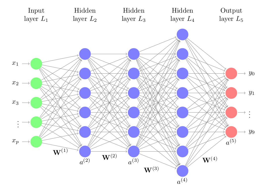
Neural networks are models created by arranging mathematical operations following a specific structure. The most common way to represent the structure of a neural network is through the use of layers (layers), which in turn are formed by neurons (units, units or neurons). Each neuron performs a simple operation and is connected to the neurons of the previous layer and the next layer through weights, whose function is to regulate the information that propagates from one neuron to another.
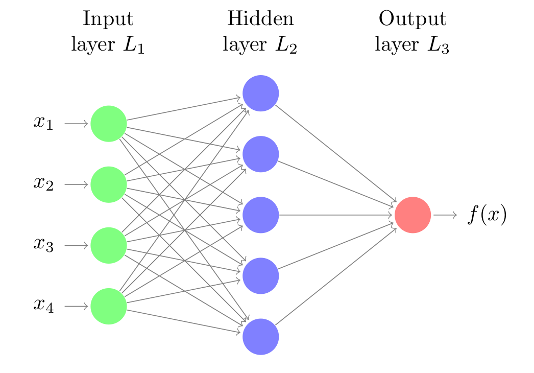
The first layer of the neural network (green color) is known as the input layer or input layer and receives the raw data, that is, the value of the predictors. The intermediate layer (blue color), known as hidden layer or hidden layer, receives the values from the input layer, weighted by the weights (gray arrows). The last layer, called output layer, combines the values that come from the intermediate layer to generate the prediction.
To facilitate understanding of network structure, it is useful to represent a network equivalent to a linear regression model.
$$y = w_1 x_1 + ... + w_d x_d + b$$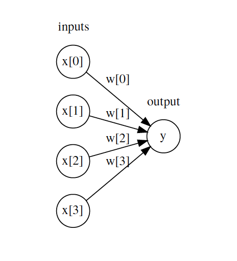
Each neuron in the input layer represents the value of one of the predictors. The arrows represent the regression coefficients, which in network terms are called weights, and the output neuron represents the predicted value. For this representation to be equivalent to the equation of a linear model, two things are missing:
The model's bias.
The multiplication and addition operations that combine the value of the predictors with the model's weights.
The intermediate layer of a network has a bias value, but it is usually omitted in graphical representations. As for the mathematical operations, this is the key element that occurs inside the neurons and it is worth seeing in detail.
The Neuron (Unit)
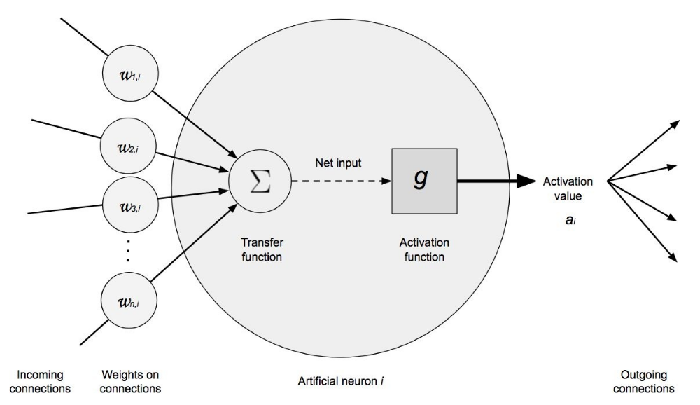
The neuron is the functional unit of network models. Within each neuron, only two operations occur: the weighted sum of its inputs and the application of an activation function.
In the first part, each input value $x_i$ is multiplied by its associated weight $w_i$ and summed together with the bias. This is the net input value to the neuron. Next, this value is passed through a function, known as an activation function, that transforms the net input value into an output value.
While the value that reaches the neuron, multiplication of weights by inputs, is always a linear combination, thanks to the activation function, very diverse outputs can be generated. It is in the activation function where the potential of network models to learn non-linear relationships resides.
The previous has been an intuitive explanation of how a neuron works. Let's now see a more mathematical definition.
The net input value to a neuron is the sum of the values that arrive, weighted by the connection weights, plus the bias.
$$entrada = \sum^n_{i=1} x_i w_i + b$$Instead of using the summation, this operation is usually represented as the matrix product, where $\textbf{X}$ represents the vector of input values and $\textbf{W}$ the weight vector.
$$entrada = \textbf{X}\textbf{W} + b$$An activation function ($g$) is applied to this value, which transforms it into what is known as the activation value ($a$), which is what finally comes out of the neuron.
$$a = g(entrada) = g(\textbf{X}\textbf{W} + b)$$For the input layer, where you only want to incorporate the value of the predictors, the activation function is the identity, that is, what comes out is the same as what goes in. In the output layer, the activation function used is usually the identity for regression problems and soft max for classification.
Activation Function
Activation functions largely control what information propagates from one layer to the next (forward propagation). These functions convert the net input value to the neuron, combination of inputs, weights and bias, into a new value. It is thanks to combining non-linear activation functions with multiple layers (see below), that network models are capable of learning non-linear relationships.
The vast majority of activation functions convert the net input value of the neuron into a value within the range (0, 1) or (-1, 1). When the activation value of a neuron (output of its activation function) is zero, the neuron is said to be inactive, since it does not pass any type of information to the following neurons. Below are the most commonly used activation functions.
Rectified linear unit (ReLU)
The ReLu activation function applies a very simple non-linear transformation, it activates the neuron only if the input is above zero. While the input value is below zero, the output value is zero, but when it is above zero, the output value increases linearly with the input.
$$\operatorname{ReLU}(x) = \max(x, 0)$$In this way, the activation function retains only positive values and discards negative ones by giving them an activation of zero.
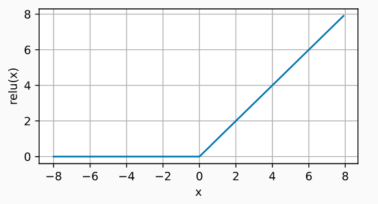
ReLU is by far the most widely used activation function, due to its good results in diverse applications. The reason for this lies in the behavior of its derivative (gradient), which is zero or constant, thus avoiding a problem known as vanishing gradients that limits the learning capacity of network models.
Sigmoid
The sigmoid function transforms values in the range (-inf, +inf) to values in the range (0, 1).
$$\operatorname{sigmoid}(x) = \frac{1}{1 + \exp(-x)}$$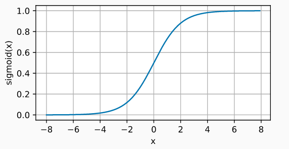
Although the sigmoid activation function was used extensively in the early days of network models, nowadays, the ReLU function is usually preferred.
One case where the sigmoid activation function is still the default function is in the output layer neurons of binary classification models, since its output can be interpreted as probabilities.
Hyperbolic Tangent (Tanh)
The Tanh activation function behaves similarly to the sigmoid function, but its output is bounded in the range (-1, 1).
$$\operatorname{tanh}(x) = \frac{1 - \exp(-2x)}{1 + \exp(-2x)}$$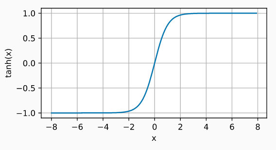
Without activation functions, neural networks can only learn linear relationships.
Loss Function (Cost Function)
The cost function ($l$), also called loss function, loss function or cost function, is the function responsible for quantifying the distance between the actual value and the value predicted by the network, in other words, it measures the error that the network makes when making predictions. In most cases, the cost function returns positive values. The closer to zero the cost value is, the better the network's predictions (lower error), being zero when the predictions exactly match the actual value.
The cost function can be calculated for a single observation or for a dataset (usually averaging the value of all observations). The second case is the one used to guide the training of models.
Depending on the type of problem, regression or classification, it is necessary to use one cost function or another. In regression problems, the most commonly used are mean squared error and mean absolute error. In classification problems, the log loss function, also called logistic loss or cross-entropy loss, is usually used.
Mean Squared Error
Mean squared error (mean squared error, MSE) is by far the most used cost function in regression problems. For a given observation $i$, the mean squared error is calculated as the difference between the predicted value $\hat{y}$ and the actual value $y$.
$$l^{(i)}(\mathbf{w}, b) = \left(\hat{y}^{(i)} - y^{(i)}\right)^2$$Cost functions are usually written with the notation $l(\mathbf{w}, b)$ to refer to the fact that their value depends on the weights and bias of the model, since these are what determine the value of the predictions $y^{(i)}$.
Frequently, this cost function is multiplied by $\frac{1}{2}$, this is simply for mathematical convenience to simplify the calculation of its derivative.
$$l^{(i)}(\mathbf{w}, b) = \frac{1}{2} \left(\hat{y}^{(i)} - y^{(i)}\right)^2$$To quantify the error that the model makes on an entire dataset, for example the training data, simply average the error of all $n$ observations.
$$L(\mathbf{w}, b) =\frac{1}{n}\sum_{i=1}^n l^{(i)}(\mathbf{w}, b) = \frac{1}{n}\sum_{i=1}^n \left(\hat{y}^{(i)} - y^{(i)}\right)^2$$When a model is trained using mean squared error as the cost function, it is learning to predict the mean of the response variable.
Mean Absolute Error
Mean absolute error (mean absolute error, MAE) consists of averaging the absolute error of predictions.
$$L(\mathbf{w}, b) =\frac{1}{n}\sum_{i=1}^n |\hat{y}^{(i)} - y^{(i)}|$$Mean absolute error is more robust to outliers than mean squared error. This means that the training of the model is less influenced by anomalous data that may be in the training set. When a model is trained using mean absolute error as the cost function, it is learning to predict the median of the response variable.
Log loss, logistic loss or cross-entropy loss
In classification problems, the output layer uses the softmax function as activation function. Thanks to this function, the network returns a series of values that can be interpreted as the probability that the predicted observation belongs to each of the possible classes.
When the classification is binary, where the response variable is 1 or 0, and $p = \operatorname{Pr}(y = 1)$, the log-likelihood cost function is defined as:
$$L_{\log}(y, p) = -\log \operatorname{Pr}(y|p) = -(y \log (p) + (1 - y) \log (1 - p))$$For classification problems with more than two classes, this formula is generalized to:
$$L_{\log}(Y, P) = -\log \operatorname{Pr}(Y|P) = - \frac{1}{N} \sum_{i=0}^{N-1} \sum_{k=0}^{K-1} y_{i,k} \log p_{i,k}$$In both cases, minimizing this function is equivalent to making the predicted probability for the correct class tend to 1, and to 0 in the other classes.
Since this function has been used in diverse fields, it is known by different names: Log loss, logistic loss or cross-entropy loss, but they all refer to the same thing. A more detailed explanation of this cost function can be found here.
Multiple Layers
The neural network model with a single layer (single-layer perceptron), although it represented a great advance in the field of machine learning, is only capable of learning simple patterns. To overcome this limitation, researchers discovered that, by combining multiple hidden layers, the network can learn much more complex relationships between predictors and the response variable. This structure is known as multilayer perceptron or multilayer perceptron (MLP), and can be considered the first deep learning model.
The structure of a multilayer perceptron consists of several layers of hidden neurons. Each neuron is connected to all neurons in the previous layer and those in the next layer. Although not strictly necessary, all neurons that are part of the same layer usually use the same activation function.
By combining multiple hidden layers and non-linear activation functions, network models can learn virtually any pattern. In fact, it has been proven that, with enough neurons, an MLP is a universal approximator for any function.
Training
The training process of a neural network consists of adjusting the value of the weights and bias in such a way that the predictions generated have the lowest possible error. Thanks to this, the model is able to identify which predictors have the greatest influence and how they are related to each other and to the response variable.
The intuitive idea of how to train a neural network is as follows:
Initialize the network with random values of weights and bias.
For each training observation ($X$, $y$), calculate the error that the network makes when making its predictions. Weight the errors of all observations.
Identify the responsibility that each weight and bias has had in the prediction error.
Slightly modify the weights and bias of the network in the correct direction to reduce the error, proportionally to their responsibility in it.
Repeat steps 2, 3, 4 and 5 until achieving acceptable performance.
While the idea seems simple, achieving a way to implement it has required the combination of multiple mathematical methods, specifically, the backpropagation algorithm (backpropagation) and gradient descent optimization (gradient descent).
In neural network models with multiple predictors, continuous predictors must always be standardized or normalized before training. This step can only be omitted when all predictors have the same scale.
Backpropagation
Backpropagation is the algorithm that allows quantifying the influence that each weight and bias of the network has on its predictions. To achieve this, it uses the chain rule (chain rule) to calculate the gradient, which is simply the vector formed by the partial derivatives of a function.
In the case of networks, the partial derivative of the error with respect to a parameter (weight or bias) measures how much "responsibility" that parameter has had in the error made. Thanks to this, it is possible to identify which weights of the network need to be modified to improve it. The next necessary step is to determine how much and how to modify them (optimization).
Gradient Descent
Gradient descent (gradient descent) is an optimization algorithm that allows minimizing a function by making updates of its parameters in the direction of the negative value of its gradient. Applied to neural networks, gradient descent allows updating the weights and biases of the model to reduce its error.
Since calculating the model's error for all training observations in each iteration can be computationally very expensive, there is an alternative to the gradient descent method called stochastic gradient (stochastic gradient descent, SGD). This method consists of dividing the training set into batches (minibatch or batch) and updating the network parameters with each one. This way, instead of waiting to evaluate all observations to update the parameters, they can be updated progressively. A complete round of iterations over all batches is called an epoch. The number of epochs with which a network is trained is equivalent to the number of times the network sees each training example.
Preprocessing
When training models based on neural networks, it is necessary to perform two types of transformations on the data.
Binarization (One hot encoding) of categorical variables
Binarization (one-hot-encoding) consists of creating new dummy variables with each of the levels of the qualitative variables. For example, a variable called color that contains the levels red, green and blue, will become three new variables (color_red, color_green, color_blue), all with value 0 except the one that matches the observation, which takes value 1.
Standardization and scaling of numerical variables
When predictors are numerical, the scale in which they are measured, as well as the magnitude of their variance can greatly influence the model. If predictors are not equalized in some way, those measured on a larger scale or with more variance will dominate the model even if they are not the ones most related to the response variable. There are mainly 2 strategies to avoid this:
Centering: consists of subtracting from each value the mean of the predictor to which it belongs. If the data is stored in a dataframe, centering is achieved by subtracting from each value the mean of the column in which it is located. As a result of this transformation, all predictors have a mean of zero, that is, the values are centered around the origin.
Normalization (standardization): consists of transforming the data so that all predictors are approximately on the same scale.
Z-score normalization (StandardScaler): divide each predictor by its standard deviation after being centered, this way, the data has a normal distribution.
Max-min standardization (MinMaxScaler): transform the data so that it is within the range [0, 1].
Variables should never be standardized after being binarized, as this would destroy the information encoded in the values 0 and 1.
Hyperparameters
The great "flexibility" that neural networks have is a double-edged sword. On one hand, they are capable of generating models that learn very complex relationships; however, they easily suffer from the problem of overfitting (overfitting) which renders them unable to predict new observations. The way to minimize this problem and achieve useful models is by properly configuring their hyperparameters. Some of the most important ones are:
Number and Size of Layers
The architecture of a network, the number of layers and the number of neurons that are part of each layer, largely determine the complexity of the model and thus its potential learning capacity.
The input and output layers are simple to establish. The input layer has as many neurons as predictors and the output layer has one neuron in regression problems and as many as classes in classification problems. In most implementations, these values are automatically set based on the training set. The user usually specifies only the number of intermediate (hidden) layers and their size.
The more neurons and layers, the greater the complexity of the relationships that the model can learn. However, since each neuron is connected by weights to the rest of the neurons in the adjacent layers, the number of parameters to learn increases and with it the training time.
Learning rate
The learning rate establishes how fast the parameters of a model can change as it is optimized (learns). This hyperparameter is one of the most complicated to establish, since it depends a lot on the data and interacts with the rest of hyperparameters. If the learning rate is very large, the optimization process can jump from one region to another without the model being able to learn. If, on the contrary, the learning rate is very small, the training process can take too long and not be completed. Some heuristic recommendations based on trial and error are:
Use a learning rate as small as possible as long as the training time does not exceed the available time limitations.
Do not use a constant value of learning rate throughout the training process. In general, use larger values at the beginning and smaller ones at the end.
Optimization Algorithm
Gradient descent and stochastic gradient descent were among the first optimization methods used to train neural network models. Both directly use the gradient to guide optimization. It was soon seen that this generates problems as networks increase in size (neurons and layers). In many regions of the search space, the gradient is very close to zero, which causes the optimization to stagnate in these regions. To avoid this problem, modifications of gradient descent have been developed that are capable of adapting the learning rate based on the gradient and subgradient. In this way, the learning process slows down or speeds up depending on the characteristics of the region of the search space in which they are located. Although there are many adaptations, it is usually recommended:
For small datasets: l-bfgs
For large datasets: adam or rmsprop
The choice of optimization algorithm can have a very large impact on model learning, especially in deep learning. An excellent more detailed description can be found in the free book Dive into Deep Learning.
Regularization
Regularization methods are used with the aim of reducing the overfitting (overfitting) of models. An overfitted model memorizes the training data, but is unable to correctly predict new observations.
Neural network models can be considered as overparameterized models; therefore, regularization strategies are fundamental. Among the many that exist, L1 and L2 regularization (weight decay), and dropout stand out.
L1 and L2 Penalty
The objective of L1 and L2 penalty, the latter also known as weight decay, is to prevent weights from taking excessively high values. This way it is avoided that a few neurons dominate the behavior of the network and it is forced that features with little information (noise) have weights close to or equal to zero.
Dropout
The process consists of randomly deactivating a series of neurons during the training process. Specifically, during each training iteration, the weights of a random fraction of neurons per layer are set to zero. The dropout method, described by Srivastava et al. in 2014, has become a standard for training neural networks. The percentage of neurons that are usually deactivated per layer (dropout rate) is usually a value between 0.2 and 0.5.
Neural Network Models in Scikit-learn
To create models based on neural networks with scikit-learn, the classes sklearn.neural_network.MLPRegressor for regression and sklearn.neural_network.MLPClassifier for classification are used.
There are many arguments that control the behavior of this type of models. Fortunately, those responsible for their implementation have established default values that usually work well in many scenarios. Below are the most influential ones:
hidden_layer_sizes: number and size of hidden layers. For example, (100) for a single hidden layer with 100 neurons, and (16, 16) for two hidden layers of 16 neurons each. The default value is (100,).activation: activation function of the hidden layers. It can be: {'identity', 'logistic', 'tanh', 'relu'}. The same activation function is applied to all hidden layers, different ones are not allowed. The default value is 'relu'.solver: the optimization algorithm used to learn the weights and bias of the network. It can be: {'lbfgs', 'sgd', 'adam'}. By default 'adam' is used, which usually gives the best results for datasets with thousands of observations. For small datasets, 'lbfgs' converges faster and can achieve better results.alpha: L2 regularization (weight decay). The default value is 0.0001.batch_size: batch size used in stochasticsolvers('sgd' and 'adam'). This parameter is ignored if the solver is 'lbfgs'. By defaultmin(200, n_samples)is used.learning_rate: strategy to modify the learning rate during training. Only used whensolver='sgd'. It can be:'constant': the value specified in the
learning_rate_initargument is used throughout the training process.'invscaling': the learning rate is progressively reduced in each iteration t using an exponential function
effective_learning_rate = learning_rate_init / pow(t, power_t).adaptive: keeps the value specified in thelearning_rate_initargument constant as long as the model continues improving (reduction of the cost function). If between two consecutive epochs the model does not improve by a minimum defined in thetolargument, the learning rate is divided by 5.
learning_rate_init: initial value of learning rate. Only used when thesolveris 'sgd' or 'adam'. The default value is 0.001.power_t: exponent used to reduce the learning rate whenlearning_rate='invscaling'. The default value is 0.5. This argument is only used whensolver='sgd'.max_iter: maximum number of training iterations. For stochastic solvers ('sgd' and 'adam') this value corresponds to the number of epochs (how many times each observation participates in training). By default 200 are used.shuffle: whether to randomly shuffle observations in each iteration. By default it isTrue.random_state: seed used for all training steps that require random values (weight initialization, splits, bias).tol: tolerance value used in optimization. If the cost function does not improve forn_iter_no_changeconsecutive iterations by a minimum oftol, training ends. By default 1e-4 is used.
early_stopping: stop training when the validation metric does not improve. Automatically, a percentage ofvalidation_fractionof the training set is separated and used as a validation set. If during more thann_iter_no_changeiterations (epochs), the validation metric does not improve by a minimum oftol, training ends. Only applies ifsolveris 'sgd' or 'adam'.validation_fraction: fraction of data from the training set used as validation set for early stopping. By default 0.1 is used.
n_iter_no_change: number of consecutive epochs without improvement that triggers early stopping. By default 10 are used.
A more detailed description of how to use the many functionalities offered by this library can be found in the article Machine learning with Python and Scikit-learn.
Classification Example
This first example shows how, depending on the architecture (hidden layers and their size), a model based on neural networks can learn non-linear functions with great ease. To avoid overfitting problems, it is important to identify the combination of hyperparameters that achieves an appropriate balance in learning. This is a very simple example, whose objective is for the reader to become familiar with the flexibility that this type of models have and how to perform a hyperparameter search using grid search and cross-validation.
Libraries
The libraries used in this example are:
# Data processing
# ==============================================================================
import numpy as np
import pandas as pd
# Plots
# ==============================================================================
import matplotlib.pyplot as plt
import seaborn as sns
plt.style.use('fivethirtyeight')
plt.rcParams.update({'font.size': 10})
# Modeling
# ==============================================================================
from sklearn.datasets import make_blobs
from sklearn.neural_network import MLPClassifier
from sklearn.model_selection import RandomizedSearchCV
from sklearn.model_selection import GridSearchCV
import multiprocessing
# Warnings configuration
# ==============================================================================
import warnings
warnings.filterwarnings('ignore')
Data
Observations are simulated in two dimensions, belonging to three groups, whose separation is not perfect.
# Simulated data
# ==============================================================================
X, y = make_blobs(
n_samples = 500,
n_features = 2,
centers = 3,
cluster_std = 1.2,
shuffle = True,
random_state = 0
)
fig, ax = plt.subplots(1, 1, figsize=(5, 5))
for i in np.unique(y):
ax.scatter(
x = X[y == i, 0],
y = X[y == i, 1],
c = plt.rcParams['axes.prop_cycle'].by_key()['color'][i],
marker = 'o',
edgecolor = 'black',
label= f"Group {i}"
)
ax.set_title('Simulated Data')
ax.legend();

Network Architecture
4 models are created in increasing order of complexity (number of neurons and layers), to verify how the network architecture affects its learning capacity.
# Models
# ==============================================================================
model_1 = MLPClassifier(
hidden_layer_sizes=(5,),
learning_rate_init=0.01,
solver = 'lbfgs',
max_iter = 1000,
random_state = 123
)
model_2 = MLPClassifier(
hidden_layer_sizes=(10,),
learning_rate_init=0.01,
solver = 'lbfgs',
max_iter = 1000,
random_state = 123
)
model_3 = MLPClassifier(
hidden_layer_sizes=(20, 20),
learning_rate_init=0.01,
solver = 'lbfgs',
max_iter = 5000,
random_state = 123
)
model_4 = MLPClassifier(
hidden_layer_sizes=(50, 50, 50),
learning_rate_init=0.01,
solver = 'lbfgs',
max_iter = 5000,
random_state = 123
)
model_1.fit(X=X, y=y)
model_2.fit(X=X, y=y)
model_3.fit(X=X, y=y)
model_4.fit(X=X, y=y)
MLPClassifier(hidden_layer_sizes=(50, 50, 50), learning_rate_init=0.01,
max_iter=5000, random_state=123, solver='lbfgs')In a Jupyter environment, please rerun this cell to show the HTML representation or trust the notebook. On GitHub, the HTML representation is unable to render, please try loading this page with nbviewer.org.
Parameters
| hidden_layer_sizes | (50, ...) | |
| activation | 'relu' | |
| solver | 'lbfgs' | |
| alpha | 0.0001 | |
| batch_size | 'auto' | |
| learning_rate | 'constant' | |
| learning_rate_init | 0.01 | |
| power_t | 0.5 | |
| max_iter | 5000 | |
| shuffle | True | |
| random_state | 123 | |
| tol | 0.0001 | |
| verbose | False | |
| warm_start | False | |
| momentum | 0.9 | |
| nesterovs_momentum | True | |
| early_stopping | False | |
| validation_fraction | 0.1 | |
| beta_1 | 0.9 | |
| beta_2 | 0.999 | |
| epsilon | 1e-08 | |
| n_iter_no_change | 10 | |
| max_fun | 15000 |
# Predictions plot
# ==============================================================================
fig, axs = plt.subplots(2, 2, figsize=(9,7))
axs = axs.flatten()
grid_x1 = np.linspace(start=min(X[:, 0]), stop=max(X[:, 0]), num=100)
grid_x2 = np.linspace(start=min(X[:, 1]), stop=max(X[:, 1]), num=100)
xx, yy = np.meshgrid(grid_x1, grid_x2)
X_grid = np.column_stack([xx.flatten(), yy.flatten()])
for i, model in enumerate([model_1, model_2, model_3, model_4]):
predictions = model.predict(X_grid)
for j in np.unique(predictions):
axs[i].scatter(
x = X_grid[predictions == j, 0],
y = X_grid[predictions == j, 1],
c = plt.rcParams['axes.prop_cycle'].by_key()['color'][j],
alpha = 0.3,
label= f"Group {j}"
)
for j in np.unique(y):
axs[i].scatter(
x = X[y == j, 0],
y = X[y == j, 1],
c = plt.rcParams['axes.prop_cycle'].by_key()['color'][j],
marker = 'o',
edgecolor = 'black'
)
axs[i].set_title(f"Hidden layers: {model.hidden_layer_sizes}")
axs[i].axis('off')
axs[0].legend()
plt.suptitle('Decision regions by neural network architecture', fontsize=16)
plt.tight_layout();

It can be observed how, as the complexity of the network increases (more neurons and more layers), the decision boundaries adapt more and more to the training data.
Hyperparameter Optimization
This section shows how some of the most influential hyperparameters affect learning. Since the two predictors have the same scale, it is not strictly necessary to apply normalization before training.
# Number of neurons
# ==============================================================================
param_grid = {'hidden_layer_sizes':[1, 5, 10, 15, 25, 50]}
grid = GridSearchCV(
estimator = MLPClassifier(
learning_rate_init = 0.01,
solver = 'lbfgs',
alpha = 0,
max_iter = 5000,
random_state = 123
),
param_grid = param_grid,
scoring = 'accuracy',
cv = 5,
refit = True,
return_train_score = True
)
_ = grid.fit(X, y)
# Error evolution as a function of number of neurons
# ==============================================================================
fig, ax = plt.subplots(figsize=(6, 3.84))
scores = pd.DataFrame(grid.cv_results_)
scores.plot(x='param_hidden_layer_sizes', y='mean_train_score', yerr='std_train_score', ax=ax)
scores.plot(x='param_hidden_layer_sizes', y='mean_test_score', yerr='std_test_score', ax=ax)
ax.set_ylabel('accuracy')
ax.set_xlabel('number of neurons')
ax.set_title('Cross-validation error');

# Learning rate
# ==============================================================================
param_grid = {'learning_rate_init':[0.0001, 0.001, 0.01, 0.1, 1, 10, 100]}
grid = GridSearchCV(
estimator = MLPClassifier(
hidden_layer_sizes=(10),
solver = 'adam',
alpha = 0,
max_iter = 5000,
random_state = 123
),
param_grid = param_grid,
scoring = 'accuracy',
cv = 5,
refit = True,
return_train_score = True
)
_ = grid.fit(X, y)
# Error evolution as a function of number of neurons
# ==============================================================================
fig, ax = plt.subplots(figsize=(6, 3.84))
scores = pd.DataFrame(grid.cv_results_)
scores.plot(x='param_learning_rate_init', y='mean_train_score', yerr='std_train_score', ax=ax)
scores.plot(x='param_learning_rate_init', y='mean_test_score', yerr='std_test_score', ax=ax)
ax.set_xscale('log')
ax.set_xlabel('log(learning rate)')
ax.set_ylabel('accuracy')
ax.set_title('Cross-validation error');

While the previous two examples serve to have an intuitive idea of how each hyperparameter affects, it is not possible to optimize them individually, since the final impact that each one has depends on what value the others take. The hyperparameter search must be done jointly.
Given the high number of hyperparameters that neural network models have, the combination of possible configurations is very high. This makes hyperparameter search by Cartesian grid search (all combinations) impractical. Instead, random grid search is usually used, which searches for random combinations. For more information about this and other search strategies, consult Hyperparameters (tuning)).
# Search space for each hyperparameter
# ==============================================================================
param_distributions = {
'hidden_layer_sizes': [(10,), (10, 10), (20, 20)],
'alpha': np.logspace(-3, 3, 7),
'learning_rate_init': [0.001, 0.01, 0.1],
}
# Cross-validation search
# ==============================================================================
grid = RandomizedSearchCV(
estimator = MLPClassifier(solver = 'lbfgs', max_iter= 2000),
param_distributions = param_distributions,
n_iter = 50, # Maximum number of combinations tested
scoring = 'accuracy',
n_jobs = multiprocessing.cpu_count() - 1,
cv = 3,
verbose = 0,
random_state = 123,
return_train_score = True
)
grid.fit(X = X, y = y)
# Grid results
# ==============================================================================
results = pd.DataFrame(grid.cv_results_)
results.filter(regex = '(param.*|mean_t|std_t)')\
.drop(columns = 'params')\
.sort_values('mean_test_score', ascending = False)\
.head(10)
| param_learning_rate_init | param_hidden_layer_sizes | param_alpha | mean_test_score | std_test_score | mean_train_score | std_train_score | |
|---|---|---|---|---|---|---|---|
| 30 | 0.010 | (10,) | 10.0 | 0.873915 | 0.040374 | 0.875981 | 0.019150 |
| 46 | 0.010 | (10,) | 100.0 | 0.869899 | 0.042016 | 0.873973 | 0.021077 |
| 49 | 0.100 | (10,) | 100.0 | 0.869899 | 0.042016 | 0.873973 | 0.021077 |
| 41 | 0.001 | (10,) | 10.0 | 0.867915 | 0.032517 | 0.875975 | 0.022360 |
| 1 | 0.001 | (10, 10) | 10.0 | 0.867915 | 0.040386 | 0.876979 | 0.020177 |
| 3 | 0.010 | (10, 10) | 1.0 | 0.867915 | 0.040386 | 0.894973 | 0.022163 |
| 4 | 0.010 | (20, 20) | 10.0 | 0.865919 | 0.037716 | 0.878978 | 0.023269 |
| 34 | 0.100 | (10, 10) | 10.0 | 0.865919 | 0.041054 | 0.879979 | 0.021889 |
| 11 | 0.001 | (10,) | 1.0 | 0.865883 | 0.052250 | 0.889974 | 0.025252 |
| 7 | 0.010 | (10, 10) | 10.0 | 0.863923 | 0.038326 | 0.882982 | 0.023467 |
The combination of hyperparameters that achieves the best results is:
# Best model
# ==============================================================================
model = grid.best_estimator_
model
MLPClassifier(alpha=np.float64(10.0), hidden_layer_sizes=(10,),
learning_rate_init=0.01, max_iter=2000, solver='lbfgs')In a Jupyter environment, please rerun this cell to show the HTML representation or trust the notebook. On GitHub, the HTML representation is unable to render, please try loading this page with nbviewer.org.
Parameters
| hidden_layer_sizes | (10,) | |
| activation | 'relu' | |
| solver | 'lbfgs' | |
| alpha | np.float64(10.0) | |
| batch_size | 'auto' | |
| learning_rate | 'constant' | |
| learning_rate_init | 0.01 | |
| power_t | 0.5 | |
| max_iter | 2000 | |
| shuffle | True | |
| random_state | None | |
| tol | 0.0001 | |
| verbose | False | |
| warm_start | False | |
| momentum | 0.9 | |
| nesterovs_momentum | True | |
| early_stopping | False | |
| validation_fraction | 0.1 | |
| beta_1 | 0.9 | |
| beta_2 | 0.999 | |
| epsilon | 1e-08 | |
| n_iter_no_change | 10 | |
| max_fun | 15000 |
Once the model is trained, since there are only two predictors, the learned classification regions can be displayed graphically.
# Final model decision regions
# ==============================================================================
grid_x1 = np.linspace(start=min(X[:, 0]), stop=max(X[:, 0]), num=100)
grid_x2 = np.linspace(start=min(X[:, 1]), stop=max(X[:, 1]), num=100)
xx, yy = np.meshgrid(grid_x1, grid_x2)
X_grid = np.column_stack([xx.flatten(), yy.flatten()])
predictions = model.predict(X_grid)
fig, ax = plt.subplots(1, 1, figsize=(5, 5))
for i in np.unique(predictions):
ax.scatter(
x = X_grid[predictions == i, 0],
y = X_grid[predictions == i, 1],
c = plt.rcParams['axes.prop_cycle'].by_key()['color'][i],
alpha = 0.3,
label= f"Group {i}"
)
for i in np.unique(y):
ax.scatter(
x = X[y == i, 0],
y = X[y == i, 1],
c = plt.rcParams['axes.prop_cycle'].by_key()['color'][i],
marker = 'o',
edgecolor = 'black'
)
ax.set_title('Classification Regions')
ax.legend();

Use Case: Housing Price Prediction
The SaratogaHouses dataset from the mosaicData package in R contains information about the price of 1728 homes located in Saratoga County, New York, USA in 2006. In addition to price, it includes 15 additional variables:
- price: house price.
- lotSize: square feet of the house.
- age: age of the house.
- landValue: land value.
- livingArea: habitable square feet.
- pctCollege: percentage of neighborhood with college degree.
- bedrooms: number of bedrooms.
- fireplaces: number of fireplaces.
- bathrooms: number of bathrooms (value 0.5 refers to bathrooms without shower).
- rooms: number of rooms.
- heating: type of heating.
- fuel: type of heating fuel (gas, electricity or diesel).
- sewer: type of drainage.
- waterfront: whether the house has lake views.
- newConstruction: whether the house is newly constructed.
- centralAir: whether the house has air conditioning.
The objective is to obtain a model capable of predicting the house price.
Libraries
# Data processing
# ==============================================================================
import numpy as np
import pandas as pd
# Plots
# ==============================================================================
import matplotlib.pyplot as plt
import seaborn as sns
%matplotlib inline
plt.style.use('fivethirtyeight')
plt.rcParams.update({'font.size': 10})
# Modeling
# ==============================================================================
from sklearn.neural_network import MLPRegressor
from sklearn.compose import ColumnTransformer
from sklearn.preprocessing import OneHotEncoder
from sklearn.preprocessing import StandardScaler
from sklearn.pipeline import Pipeline
from sklearn.metrics import root_mean_squared_error
from sklearn.model_selection import RandomizedSearchCV
from sklearn.model_selection import train_test_split
import multiprocessing
# Warnings configuration
# ==============================================================================
import warnings
warnings.filterwarnings('ignore')
Data
# Data download
# ==============================================================================
url = ("https://raw.githubusercontent.com/JoaquinAmatRodrigo/"
"Estadistica-machine-learning-python/master/data/SaratogaHouses.csv")
data = pd.read_csv(url, sep=",")
# Columns are renamed to be more descriptive
data.columns = ["price", "total_sqft", "age", "land_value",
"living_area", "pct_college", "bedrooms",
"fireplace", "bathrooms", "rooms", "heating",
"fuel", "sewer", "waterfront",
"new_construction", "central_air"]
Exploratory Analysis
Before training a predictive model, or even before performing any calculation with a new dataset, it is very important to perform a descriptive exploration of it. This process allows better understanding of what information each variable contains, as well as detecting possible errors. Some frequent examples are:
That a column has been stored with the incorrect type: a numerical variable is being recognized as text or vice versa.
That a variable contains values that do not make sense: for example, to indicate that the price of a house is not available, the value 0 or a blank space is entered.
That a word has been entered in a numerical variable instead of a number.
In addition, this initial analysis can give clues about which variables are suitable as predictors in a model.
# Type of each column
# ==============================================================================
# In pandas, the "object" type refers to strings
data.info()
<class 'pandas.core.frame.DataFrame'> RangeIndex: 1728 entries, 0 to 1727 Data columns (total 16 columns): # Column Non-Null Count Dtype --- ------ -------------- ----- 0 price 1728 non-null int64 1 total_sqft 1728 non-null float64 2 age 1728 non-null int64 3 land_value 1728 non-null int64 4 living_area 1728 non-null int64 5 pct_college 1728 non-null int64 6 bedrooms 1728 non-null int64 7 fireplace 1728 non-null int64 8 bathrooms 1728 non-null float64 9 rooms 1728 non-null int64 10 heating 1728 non-null object 11 fuel 1728 non-null object 12 sewer 1728 non-null object 13 waterfront 1728 non-null object 14 new_construction 1728 non-null object 15 central_air 1728 non-null object dtypes: float64(2), int64(8), object(6) memory usage: 216.1+ KB
All columns have the correct data type.
# Number of missing data per variable
# ==============================================================================
data.isna().sum().sort_values()
price 0 total_sqft 0 age 0 land_value 0 living_area 0 pct_college 0 bedrooms 0 fireplace 0 bathrooms 0 rooms 0 heating 0 fuel 0 sewer 0 waterfront 0 new_construction 0 central_air 0 dtype: int64
All columns are complete, there are no missing values.
# Response variable distribution
# ==============================================================================
fig, ax = plt.subplots(nrows=1, ncols=1, figsize=(6, 3))
sns.histplot(data=data, x='price', kde=True,ax=ax)
ax.set_title("Price Distribution")
ax.set_xlabel('price');

Neural network models are non-parametric, they do not assume any type of distribution of the response variable, therefore, it is not necessary for it to follow any specific distribution (normal, gamma...). Even so, it is always advisable to do a minimum study, since, after all, it is what we are interested in predicting. In this case, the price variable has an asymmetric distribution with a positive tail because a few houses have a price much higher than the average.
# Distribution plot for each numerical variable
# ==============================================================================
fig, axes = plt.subplots(nrows=3, ncols=3, figsize=(9, 7))
axes = axes.flat
numeric_cols = data.select_dtypes(include=['float64', 'int']).columns
numeric_cols = numeric_cols.drop('price')
for i, colum in enumerate(numeric_cols):
sns.histplot(
data = data,
x = colum,
stat = "count",
kde = True,
color = (list(plt.rcParams['axes.prop_cycle'])*2)[i]["color"],
line_kws= {'linewidth': 2},
alpha = 0.3,
ax = axes[i]
)
axes[i].set_title(colum, fontsize = 7)
axes[i].tick_params(labelsize = 6)
axes[i].set_xlabel("")
axes[i].set_ylabel("")
fig.tight_layout()
plt.subplots_adjust(top = 0.9)
fig.suptitle('Numerical variables distribution', fontsize = 10, fontweight = "bold");

The fireplace variable, although numeric, takes only a few values and the vast majority of observations belong to only two of them. In cases like this, it is usually convenient to treat the variable as qualitative.
# Observed values of fireplace
# ==============================================================================
data.fireplace = data.fireplace.astype("str")
data.fireplace.value_counts()
fireplace 1 942 0 740 2 42 4 2 3 2 Name: count, dtype: int64
# Qualitative variables (object type)
# ==============================================================================
data.select_dtypes(include=['object']).describe()
| fireplace | heating | fuel | sewer | waterfront | new_construction | central_air | |
|---|---|---|---|---|---|---|---|
| count | 1728 | 1728 | 1728 | 1728 | 1728 | 1728 | 1728 |
| unique | 5 | 3 | 3 | 3 | 2 | 2 | 2 |
| top | 1 | hot air | gas | public/commercial | No | No | No |
| freq | 942 | 1121 | 1197 | 1213 | 1713 | 1647 | 1093 |
# Plot for each qualitative variable
# ==============================================================================
fig, axes = plt.subplots(nrows=3, ncols=3, figsize=(9, 5))
axes = axes.flat
object_cols = data.select_dtypes(include=['object']).columns
for i, colum in enumerate(object_cols):
data[colum].value_counts().plot.barh(ax = axes[i])
axes[i].set_title(colum, fontsize = 12)
axes[i].set_xlabel("")
# Remove empty axes
for i in [7, 8]:
fig.delaxes(axes[i])
fig.tight_layout()

If any of the levels of a qualitative variable has very few observations compared to the other levels, it can happen that, during cross-validation or bootstrapping, some partitions do not contain any observation of that class (zero variance), which can lead to errors. For this case, caution should be taken with the fireplace variable. Levels 2, 3 and 4 are merged into a new level called "2_plus".
replace_dict = {'2': "2_plus",
'3': "2_plus",
'4': "2_plus"}
data['fireplace'] = data['fireplace'] \
.map(replace_dict) \
.fillna(data['fireplace'])
data.fireplace.value_counts().sort_index()
fireplace 0 740 1 942 2_plus 46 Name: count, dtype: int64
Train and Test Split
In order to estimate the error that the model makes when predicting new observations, the data is divided into two groups, one for training and another for testing (80%, 20%).
# Train and test data split
# ==============================================================================
X_train, X_test, y_train, y_test = train_test_split(
data.drop('price', axis = 'columns'),
data['price'],
train_size = 0.8,
random_state = 1234,
shuffle = True
)
After making the split, it is verified that the two groups are similar.
print("Training partition")
print("-----------------------")
display(y_train.describe())
display(X_train.describe())
display(X_train.describe(include = 'object'))
print(" ")
print("Test partition")
print("-----------------------")
display(y_test.describe())
display(X_test.describe())
display(X_test.describe(include = 'object'))
Training partition -----------------------
count 1382.000000 mean 211436.516643 std 96846.639129 min 10300.000000 25% 145625.000000 50% 190000.000000 75% 255000.000000 max 775000.000000 Name: price, dtype: float64
| total_sqft | age | land_value | living_area | pct_college | bedrooms | bathrooms | rooms | |
|---|---|---|---|---|---|---|---|---|
| count | 1382.000000 | 1382.000000 | 1382.000000 | 1382.000000 | 1382.000000 | 1382.000000 | 1382.000000 | 1382.000000 |
| mean | 0.501331 | 27.494211 | 34232.141823 | 1755.940666 | 55.439942 | 3.165702 | 1.902677 | 7.073082 |
| std | 0.671766 | 28.212721 | 35022.662319 | 621.262215 | 10.356656 | 0.825487 | 0.660053 | 2.315395 |
| min | 0.000000 | 0.000000 | 200.000000 | 616.000000 | 20.000000 | 1.000000 | 0.000000 | 2.000000 |
| 25% | 0.170000 | 13.000000 | 15100.000000 | 1302.000000 | 52.000000 | 3.000000 | 1.500000 | 5.000000 |
| 50% | 0.370000 | 19.000000 | 25000.000000 | 1650.000000 | 57.000000 | 3.000000 | 2.000000 | 7.000000 |
| 75% | 0.540000 | 33.750000 | 39200.000000 | 2127.250000 | 63.000000 | 4.000000 | 2.500000 | 9.000000 |
| max | 8.970000 | 201.000000 | 412600.000000 | 4856.000000 | 82.000000 | 7.000000 | 4.500000 | 12.000000 |
| fireplace | heating | fuel | sewer | waterfront | new_construction | central_air | |
|---|---|---|---|---|---|---|---|
| count | 1382 | 1382 | 1382 | 1382 | 1382 | 1382 | 1382 |
| unique | 3 | 3 | 3 | 3 | 2 | 2 | 2 |
| top | 1 | hot air | gas | public/commercial | No | No | No |
| freq | 741 | 915 | 972 | 970 | 1370 | 1321 | 863 |
Test partition -----------------------
count 346.000000 mean 214084.395954 std 104689.155889 min 5000.000000 25% 139000.000000 50% 180750.000000 75% 271750.000000 max 670000.000000 Name: price, dtype: float64
| total_sqft | age | land_value | living_area | pct_college | bedrooms | bathrooms | rooms | |
|---|---|---|---|---|---|---|---|---|
| count | 346.000000 | 346.000000 | 346.000000 | 346.000000 | 346.000000 | 346.000000 | 346.000000 | 346.000000 |
| mean | 0.495751 | 29.601156 | 35855.491329 | 1751.121387 | 56.078035 | 3.109827 | 1.890173 | 6.916185 |
| std | 0.798240 | 32.884116 | 35035.761216 | 615.486848 | 10.239861 | 0.783575 | 0.652368 | 2.319776 |
| min | 0.010000 | 0.000000 | 300.000000 | 792.000000 | 20.000000 | 1.000000 | 1.000000 | 2.000000 |
| 25% | 0.160000 | 13.000000 | 15100.000000 | 1296.000000 | 52.000000 | 3.000000 | 1.500000 | 5.000000 |
| 50% | 0.370000 | 19.000000 | 26700.000000 | 1608.000000 | 57.000000 | 3.000000 | 2.000000 | 7.000000 |
| 75% | 0.557500 | 34.000000 | 45950.000000 | 2181.000000 | 64.000000 | 4.000000 | 2.500000 | 8.000000 |
| max | 12.200000 | 225.000000 | 233000.000000 | 5228.000000 | 82.000000 | 6.000000 | 4.000000 | 12.000000 |
| fireplace | heating | fuel | sewer | waterfront | new_construction | central_air | |
|---|---|---|---|---|---|---|---|
| count | 346 | 346 | 346 | 346 | 346 | 346 | 346 |
| unique | 3 | 3 | 3 | 3 | 2 | 2 | 2 |
| top | 1 | hot air | gas | public/commercial | No | No | No |
| freq | 201 | 206 | 225 | 243 | 343 | 326 | 230 |
Preprocessing
Neural network models require at least two types of preprocessing: binarization (One hot encoding) of categorical variables and standardization of continuous variables.
# Variable selection by type
# ==============================================================================
# Numerical columns are standardized and one-hot-encoding is applied to
# qualitative columns. To keep columns to which no transformation is applied,
# remainder='passthrough' must be indicated.
# Identification of numerical and categorical columns
numeric_cols = X_train.select_dtypes(include=['float64', 'int']).columns.to_list()
cat_cols = X_train.select_dtypes(include=['object', 'category']).columns.to_list()
# Transformations for numerical variables
numeric_transformer = Pipeline(
steps=[('scaler', StandardScaler())]
)
# Transformations for categorical variables
categorical_transformer = Pipeline(
steps=[('onehot', OneHotEncoder(handle_unknown='ignore', sparse_output=False))]
)
preprocessor = ColumnTransformer(
transformers=[
('numeric', numeric_transformer, numeric_cols),
('cat', categorical_transformer, cat_cols)
],
remainder='passthrough'
).set_output(transform="pandas")
preprocessor
ColumnTransformer(remainder='passthrough',
transformers=[('numeric',
Pipeline(steps=[('scaler', StandardScaler())]),
['total_sqft', 'age', 'land_value',
'living_area', 'pct_college', 'bedrooms',
'bathrooms', 'rooms']),
('cat',
Pipeline(steps=[('onehot',
OneHotEncoder(handle_unknown='ignore',
sparse_output=False))]),
['fireplace', 'heating', 'fuel', 'sewer',
'waterfront', 'new_construction',
'central_air'])])In a Jupyter environment, please rerun this cell to show the HTML representation or trust the notebook. On GitHub, the HTML representation is unable to render, please try loading this page with nbviewer.org.
Parameters
| transformers | [('numeric', ...), ('cat', ...)] | |
| remainder | 'passthrough' | |
| sparse_threshold | 0.3 | |
| n_jobs | None | |
| transformer_weights | None | |
| verbose | False | |
| verbose_feature_names_out | True | |
| force_int_remainder_cols | 'deprecated' |
['total_sqft', 'age', 'land_value', 'living_area', 'pct_college', 'bedrooms', 'bathrooms', 'rooms']
Parameters
| copy | True | |
| with_mean | True | |
| with_std | True |
['fireplace', 'heating', 'fuel', 'sewer', 'waterfront', 'new_construction', 'central_air']
Parameters
| categories | 'auto' | |
| drop | None | |
| sparse_output | False | |
| dtype | <class 'numpy.float64'> | |
| handle_unknown | 'ignore' | |
| min_frequency | None | |
| max_categories | None | |
| feature_name_combiner | 'concat' |
passthrough
# Preprocessing transformations are learned and applied
# ==============================================================================
X_train_prep = preprocessor.fit_transform(X_train)
X_test_prep = preprocessor.transform(X_test)
X_train_prep.info()
<class 'pandas.core.frame.DataFrame'> Index: 1382 entries, 1571 to 815 Data columns (total 26 columns): # Column Non-Null Count Dtype --- ------ -------------- ----- 0 numeric__total_sqft 1382 non-null float64 1 numeric__age 1382 non-null float64 2 numeric__land_value 1382 non-null float64 3 numeric__living_area 1382 non-null float64 4 numeric__pct_college 1382 non-null float64 5 numeric__bedrooms 1382 non-null float64 6 numeric__bathrooms 1382 non-null float64 7 numeric__rooms 1382 non-null float64 8 cat__fireplace_0 1382 non-null float64 9 cat__fireplace_1 1382 non-null float64 10 cat__fireplace_2_plus 1382 non-null float64 11 cat__heating_electric 1382 non-null float64 12 cat__heating_hot air 1382 non-null float64 13 cat__heating_hot water/steam 1382 non-null float64 14 cat__fuel_electric 1382 non-null float64 15 cat__fuel_gas 1382 non-null float64 16 cat__fuel_oil 1382 non-null float64 17 cat__sewer_none 1382 non-null float64 18 cat__sewer_public/commercial 1382 non-null float64 19 cat__sewer_septic 1382 non-null float64 20 cat__waterfront_No 1382 non-null float64 21 cat__waterfront_Yes 1382 non-null float64 22 cat__new_construction_No 1382 non-null float64 23 cat__new_construction_Yes 1382 non-null float64 24 cat__central_air_No 1382 non-null float64 25 cat__central_air_Yes 1382 non-null float64 dtypes: float64(26) memory usage: 291.5 KB
While performing preprocessing separately from training is useful for exploring and confirming that the transformations performed are as desired, in practice, it is more appropriate to associate it with the training process itself. This can be easily done in scikit-learn models with Pipeline.
Modeling
Preprocessing + modeling Pipeline
# Preprocessing and modeling pipeline
# ==============================================================================
# Identification of numerical and categorical columns
numeric_cols = X_train.select_dtypes(include=['float64', 'int']).columns.to_list()
cat_cols = X_train.select_dtypes(include=['object', 'category']).columns.to_list()
# Transformations for numerical variables
numeric_transformer = Pipeline(
steps=[('scaler', StandardScaler())]
)
# Transformations for categorical variables
categorical_transformer = Pipeline(
steps=[('onehot', OneHotEncoder(handle_unknown='ignore', sparse_output=False))]
)
preprocessor = ColumnTransformer(
transformers=[
('numeric', numeric_transformer, numeric_cols),
('cat', categorical_transformer, cat_cols)
],
remainder='passthrough'
).set_output(transform="pandas")
# Combine preprocessing steps and model in a single pipeline
pipe = Pipeline([('preprocessing', preprocessor),
('model', MLPRegressor(solver = 'lbfgs', max_iter= 1000))])
pipe
Pipeline(steps=[('preprocessing',
ColumnTransformer(remainder='passthrough',
transformers=[('numeric',
Pipeline(steps=[('scaler',
StandardScaler())]),
['total_sqft', 'age',
'land_value', 'living_area',
'pct_college', 'bedrooms',
'bathrooms', 'rooms']),
('cat',
Pipeline(steps=[('onehot',
OneHotEncoder(handle_unknown='ignore',
sparse_output=False))]),
['fireplace', 'heating',
'fuel', 'sewer',
'waterfront',
'new_construction',
'central_air'])])),
('model', MLPRegressor(max_iter=1000, solver='lbfgs'))])In a Jupyter environment, please rerun this cell to show the HTML representation or trust the notebook. On GitHub, the HTML representation is unable to render, please try loading this page with nbviewer.org.
Parameters
| steps | [('preprocessing', ...), ('model', ...)] | |
| transform_input | None | |
| memory | None | |
| verbose | False |
Parameters
| transformers | [('numeric', ...), ('cat', ...)] | |
| remainder | 'passthrough' | |
| sparse_threshold | 0.3 | |
| n_jobs | None | |
| transformer_weights | None | |
| verbose | False | |
| verbose_feature_names_out | True | |
| force_int_remainder_cols | 'deprecated' |
['total_sqft', 'age', 'land_value', 'living_area', 'pct_college', 'bedrooms', 'bathrooms', 'rooms']
Parameters
| copy | True | |
| with_mean | True | |
| with_std | True |
['fireplace', 'heating', 'fuel', 'sewer', 'waterfront', 'new_construction', 'central_air']
Parameters
| categories | 'auto' | |
| drop | None | |
| sparse_output | False | |
| dtype | <class 'numpy.float64'> | |
| handle_unknown | 'ignore' | |
| min_frequency | None | |
| max_categories | None | |
| feature_name_combiner | 'concat' |
passthrough
Parameters
| loss | 'squared_error' | |
| hidden_layer_sizes | (100,) | |
| activation | 'relu' | |
| solver | 'lbfgs' | |
| alpha | 0.0001 | |
| batch_size | 'auto' | |
| learning_rate | 'constant' | |
| learning_rate_init | 0.001 | |
| power_t | 0.5 | |
| max_iter | 1000 | |
| shuffle | True | |
| random_state | None | |
| tol | 0.0001 | |
| verbose | False | |
| warm_start | False | |
| momentum | 0.9 | |
| nesterovs_momentum | True | |
| early_stopping | False | |
| validation_fraction | 0.1 | |
| beta_1 | 0.9 | |
| beta_2 | 0.999 | |
| epsilon | 1e-08 | |
| n_iter_no_change | 10 | |
| max_fun | 15000 |
# Search space for each hyperparameter
# ==============================================================================
param_distributions = {
'model__hidden_layer_sizes': [(10,), (20,), (10, 10)],
'model__alpha': np.logspace(-3, 3, 10),
'model__learning_rate_init': [0.001, 0.01],
}
# Cross-validation search
# ==============================================================================
grid = RandomizedSearchCV(
estimator = pipe,
param_distributions = param_distributions,
n_iter = 50,
scoring = 'neg_mean_squared_error',
n_jobs = multiprocessing.cpu_count() - 1,
cv = 5,
verbose = 0,
random_state = 123,
return_train_score = True
)
grid.fit(X = X_train, y = y_train)
# Grid results
# ==============================================================================
results = pd.DataFrame(grid.cv_results_)
results.filter(regex = '(param.*|mean_t|std_t)')\
.drop(columns = 'params')\
.sort_values('mean_test_score', ascending = False)\
.head(10)
| param_model__learning_rate_init | param_model__hidden_layer_sizes | param_model__alpha | mean_test_score | std_test_score | mean_train_score | std_train_score | |
|---|---|---|---|---|---|---|---|
| 3 | 0.010 | (10,) | 2.154435 | -3.315367e+09 | 7.678397e+08 | -2.627431e+09 | 2.278985e+08 |
| 12 | 0.001 | (10,) | 1000.000000 | -3.339797e+09 | 7.134176e+08 | -2.738077e+09 | 2.135130e+08 |
| 46 | 0.010 | (10,) | 215.443469 | -3.485172e+09 | 5.667754e+08 | -2.425853e+09 | 2.199546e+08 |
| 8 | 0.010 | (10,) | 1000.000000 | -3.495804e+09 | 5.151657e+08 | -2.635577e+09 | 1.558983e+08 |
| 26 | 0.001 | (10,) | 0.004642 | -3.506853e+09 | 7.669201e+08 | -2.527091e+09 | 1.858837e+08 |
| 41 | 0.001 | (10,) | 10.000000 | -3.516382e+09 | 6.949587e+08 | -2.726862e+09 | 1.488116e+08 |
| 9 | 0.010 | (10,) | 0.021544 | -3.531212e+09 | 8.349181e+08 | -2.596213e+09 | 2.660881e+08 |
| 4 | 0.010 | (10,) | 46.415888 | -3.553702e+09 | 7.373035e+08 | -2.499331e+09 | 1.233599e+08 |
| 20 | 0.001 | (10,) | 0.021544 | -3.556939e+09 | 6.823796e+08 | -2.593701e+09 | 2.590841e+08 |
| 32 | 0.010 | (10,) | 0.004642 | -3.564638e+09 | 6.276564e+08 | -2.706423e+09 | 2.517506e+08 |
Test Error
Although through validation methods (Kfold, LeaveOneOut) good estimates of the error that a model has when predicting new observations are obtained, the best way to evaluate a final model is by using a test set, that is, a set of observations that has been kept aside from the training and optimization process.
# Test error
# ==============================================================================
final_model = grid.best_estimator_
predictions = final_model.predict(X = X_test)
rmse = root_mean_squared_error(
y_true = y_test,
y_pred = predictions
)
print('Test error (rmse): ', rmse)
Test error (rmse): 68676.83965289967
Conclusion
The combination of hyperparameters with which the best results are obtained according to cross-validation metrics is:
final_model['model'].get_params()
{'activation': 'relu',
'alpha': np.float64(2.154434690031882),
'batch_size': 'auto',
'beta_1': 0.9,
'beta_2': 0.999,
'early_stopping': False,
'epsilon': 1e-08,
'hidden_layer_sizes': (10,),
'learning_rate': 'constant',
'learning_rate_init': 0.01,
'loss': 'squared_error',
'max_fun': 15000,
'max_iter': 1000,
'momentum': 0.9,
'n_iter_no_change': 10,
'nesterovs_momentum': True,
'power_t': 0.5,
'random_state': None,
'shuffle': True,
'solver': 'lbfgs',
'tol': 0.0001,
'validation_fraction': 0.1,
'verbose': False,
'warm_start': False}
The model's error (rmse) when applied to the test set is 60948.
Session Information
import session_info
session_info.show(html=False)
----- matplotlib 3.10.8 numpy 2.2.6 pandas 2.3.3 seaborn 0.13.2 session_info v1.0.1 sklearn 1.7.2 ----- IPython 9.8.0 jupyter_client 8.7.0 jupyter_core 5.9.1 ----- Python 3.13.11 | packaged by Anaconda, Inc. | (main, Dec 10 2025, 21:28:48) [GCC 14.3.0] Linux-6.14.0-37-generic-x86_64-with-glibc2.39 ----- Session information updated at 2025-12-26 13:47
Bibliography
The Elements of Statistical Learning (2nd edition)
Hastie, Tibshirani and Friedman (2009). Springer-Verlag.
Applied Predictive Modeling by Max Kuhn and Kjell Johnson
Deep Learning by Josh Patterson, Adam Gibson
Python Machine Learning 3rd Edition by Sebastian Raschka
Hands-On Computer Vision with TensorFlow 2 by Benjamin Planche and Eliot Andres
Citation Instructions
How to cite this document?
If you use this document or any part of it, we would appreciate a citation. Thank you very much!
Neural Networks with Python by Joaquín Amat Rodrigo, available under an Attribution-NonCommercial-ShareAlike 4.0 International (CC BY-NC-SA 4.0 DEED) license at https://cienciadedatos.net/documentos/py35-neural-networks-python.html
Did you like this article? Your support matters
Your contribution will help me continue creating free educational content. Thank you so much! 😊


This document created by Joaquín Amat Rodrigo is licensed under Attribution-NonCommercial-ShareAlike 4.0 International.
Permitted:
-
Share: copy and redistribute the material in any medium or format.
-
Adapt: remix, transform, and build upon the material.
Under the following terms:
-
Attribution: You must give appropriate credit, provide a link to the license, and indicate if changes were made. You may do so in any reasonable manner, but not in any way that suggests the licensor endorses you or your use.
-
NonCommercial: You may not use the material for commercial purposes.
-
ShareAlike: If you remix, transform, or build upon the material, you must distribute your contributions under the same license as the original.