More about machine learning: Machine Learning with Python
- Linear regression
- Logistic regression
- Decision trees
- Random forest
- Gradient boosting
- Machine learning with Python and Scikitlearn
- Neural Networks
- Principal Component Analysis (PCA)
- Clustering with python
- Face Detection and Recognition
- Introduction to Graphs and Networks
Introduction
A Gradient Boosting model is composed of a set of individual decision trees, trained sequentially, so that each new tree tries to improve on the errors of the previous ones. The prediction of a new observation is obtained by combining the predictions of all the individual trees that make up the model.
Many predictive methods generate global models in which a single equation is applied to the entire sample space. When multiple predictors are available, which interact with each other in a complex and non-linear way, it is very difficult to find a single global model that is capable of reflecting the relationship between the variables. Statistical and machine learning methods based on trees encompass a set of non-parametric supervised techniques that manage to segment the predictor space into simple regions, within which it is easier to handle interactions. This characteristic gives them a large part of their potential.
Tree-based methods have become a benchmark in the field of machine learning due to the good results they generate in very diverse problems. Throughout this document, the way in which Gradient Boosting Trees models are built and used is explored.
✏️ Note
Since the fundamental element of a Gradient Boosting Trees model is the decision tree, it is essential to understand how they work. It is also recommended to be familiar with Random Forest models, which share many characteristics with Gradient Boosting.
Advantages
They are able to select the most relevant predictors automatically.
They can be applied to regression and classification problems.
Trees can, in theory, handle both numerical and categorical predictors without having to create dummy or one-hot-encoding variables. In practice, this depends on the implementation of the algorithm in each library.
As they are non-parametric methods, they do not require the data to follow a specific distribution.
In general, they require less data cleaning and preprocessing compared to other statistical learning methods. For example, they do not require standardization.
They are less susceptible to being influenced by outliers.
If the value of a predictor is not available for an observation, a prediction can still be made using the observations from the last node reached. The accuracy of the prediction will be reduced, but at least it can be obtained.
They are very useful in data exploration, allowing for the quick and efficient identification of the most important variables (predictors).
They are suitable for datasets with a large number of observations, demonstrating good scalability.
Disadvantages
The combination of multiple trees reduces interpretability compared to models based on a single tree.
When dealing with continuous predictors, some information can be lost when categorizing them during node splitting.
As described later, the creation of tree branches is achieved through the recursive binary splitting algorithm. This algorithm identifies and evaluates possible splits for each predictor according to a certain measure (RSS, Gini, entropy...). Continuous predictors or qualitative predictors with many levels have a higher probability of containing, just by chance, some optimal cut-off point, so they are usually favored in the creation of trees.
They are not able to extrapolate outside the range observed in the training data.
Gradient Boosting in Python
Due to its good results, Gradient Boosting has become the reference algorithm when dealing with tabular data, which is why multiple implementations have been developed. All of them are highly optimized and are used in a similar way, however, they have differences in their implementation that can lead to different results.
GradientBoostingClassifierandGradientBoostingRegressor: are the first implementations of Gradient Boosting in scikit-learn.- Does not perform binning
- Uses a single core (does not parallelize any part of the algorithm)
- Allows working on sparse matrices
- Requires one-hot-encoding of categorical variables
HistGradientBoostingClassifierandHistGradientBoostingRegressor: new scikit-learn implementation largely inspired by LightGBM. According to the authors, this second implementation has many more advantages than the original, including its speed.- Performs binning
- Multicore (parallelizes some parts of the algorithm)
- Allows observations to include missing values
- Allows monotonic constraints
- No one-hot-encoding of categorical variables is necessary.
-
- Allows observations to include missing values
- Allows the use of GPUs
- Parallelized training (parallelizes some parts of the algorithm)
- Allows monotonic constraints
- Allows working on sparse matrices
- Accepts categorical variables
-
- Allows observations to include missing values
- Allows the use of GPUs
- Parallelized training (parallelizes some parts of the algorithm)
- Allows monotonic constraints
- Allows working on sparse matrices
- Accepts categorical variables
-
- Optimized mainly for categorical variables
- Uses symmetric trees
- Allows observations to include missing values
- Allows the use of GPUs
- Parallelized training (parallelizes some parts of the algorithm)
- Allows monotonic constraints
- Accepts categorical variables
-
- Performs binning
- Multicore (parallelizes some parts of the algorithm)
- Allows observations to include missing values
- Allows monotonic constraints
- Accepts categorical variables
✏️ Note
While all these libraries have a scikit-learn compatible API, some of their functionalities are not accessible this way, so for more precise use, it is recommended to use their native API.
Gradient Boosting Trees
A Gradient Boosting Trees model is formed by an ensemble of individual decision trees, trained sequentially. Each new tree uses information from the previous tree to learn from its errors, improving iteration by iteration. In each individual tree, the observations are distributed through bifurcations (nodes), generating the structure of the tree until a terminal node is reached. The prediction of a new observation is obtained by aggregating the predictions of all the individual trees that form the model.
To understand how Gradient Boosting Trees models work, it is necessary to first know the concepts of ensemble and boosting.
Ensemble methods
All statistical and machine learning models face the challenge of the bias-variance tradeoff.
The term "bias" refers to how much, on average, the predictions of a model deviate from the true values. It reflects the model's ability to capture the true relationship between the predictors and the response variable. For example, if the relationship follows a non-linear pattern, a linear regression model, regardless of how much data is available, will not be able to adequately model the relationship and will have a high bias.
On the other hand, the term "variance" refers to how much the model changes depending on the data used for its training. Ideally, a model should not change too much with small variations in the training data. If this happens, it indicates that the model is memorizing the data instead of learning the true relationship between the predictors and the response variable. For example, a tree model with many nodes tends to change its structure even with small variations in the training data, which indicates that it has high variance.
As the complexity of a model increases, it has greater flexibility to adapt to the observations, which leads to a reduction in bias and an improvement in its predictive capacity. However, once a certain level of complexity is reached, the problem of overfitting arises. This phenomenon occurs when the model fits the training data so well that it is unable to correctly predict new observations. The optimal model is one that manages to find an adequate balance between bias and variance.
How are bias and variance controlled in tree-based models? In general, small trees with few branches tend to have low variance but may not accurately capture the relationship between the variables, which translates into high bias. On the other hand, large trees fit the training data very well, which reduces bias but increases variance. One way to solve this problem is through ensemble methods.
Ensemble methods combine multiple models into a new one with the aim of achieving a balance between bias and variance, thus achieving better predictions than any of the original individual models. Two of the most used types of ensemble are:
Bagging: multiple models are fitted, each with a different subset of the training data. To predict, all the models that form the aggregate participate by contributing their prediction. As a final value, the average of all predictions (continuous variables) or the most frequent class (categorical variables) is taken. Random Forest models are in this category.
Boosting: multiple simple models, called weak learners, are fitted sequentially, so that each model learns from the errors of the previous one. In the case of Gradient Boosting Trees, weak learners are obtained by using trees with one or a few branches. As a final value, as in bagging, the average of all predictions (continuous variables) or the most frequent class (qualitative variables) is taken. Three of the most used boosting algorithms are AdaBoost, Gradient Boosting, and Stochastic Gradient Boosting. All of them are characterized by having a considerable number of hyperparameters, whose optimal value has to be identified through cross-validation. Three of the most important are:
The number of weak learners or number of iterations: unlike bagging and random forest, boosting can suffer from overfitting if this value is excessively high. To avoid this, a regularization term known as learning rate is used.
Learning rate: controls the influence that each weak learner has on the ensemble as a whole, that is, the rate at which the model learns. Values of 0.001 or 0.01 are usually recommended, although the correct choice may vary depending on the problem. The lower its value, the more trees are needed to achieve good results but the lower the risk of overfitting.
If the weak learners are trees, the maximum allowed size of each tree. Small values, between 1 and 10, are usually used.
Although the final objective is the same, to achieve an optimal balance between bias and variance, there are two important differences:
How they manage to reduce the total error. The total error of a model can be decomposed as $bias + variance + \epsilon$. In bagging, models with very low bias but high variance are used, and by aggregating them, the variance is reduced without significantly increasing the bias. In boosting, models with very low variance but high bias are used, and by sequentially fitting the models, the bias is reduced. Therefore, each of the strategies reduces a part of the total error.
How variations are introduced in the models that form the ensemble. In bagging, each model is different from the rest because each one is trained with a different sample obtained through bootstrapping). In boosting, the models are fitted sequentially and the importance (weight) of the observations changes in each iteration, giving rise to different fits.
The key for ensemble methods to achieve better results than any of their individual models is that the models that form them are as diverse as possible (their errors are not correlated). An analogy that reflects this concept is the following: suppose a game like Trivial Pursuit in which teams have to answer questions on various topics. A team made up of many players, each an expert in a different subject, will have a better chance of winning than a team made up of players who are experts in a single subject or a single player who knows a little about all the subjects.
Next, the boosting strategies, on which the Gradient Boosting Trees model is based, are described in more detail.
AdaBoost
The publication in 1995 of the AdaBoost (Adaptive Boosting) algorithm by Yoav Freund and Robert Schapire was a very important advance in the field of statistical learning, as it made it possible to apply the boosting strategy to a multitude of problems. For AdaBoost to work (binary classification problem), it is necessary to establish:
A type of model, usually called a weak learner or base learner, that is capable of predicting the response variable with a success rate slightly higher than expected by chance. In the case of regression trees, this weak learner is usually a tree with only a few nodes.
Encode the two classes of the response variable as +1 and -1.
An initial and equal weight for all observations in the training set.
Once these three points have been established, an iterative process begins. In the first iteration, the weak learner is fitted using the training data and the initial weights (all equal). With the weak learner fitted and stored, the training observations are predicted and those that are well and poorly classified are identified. With this information:
The weights of the observations are updated, decreasing the weight of those that are well classified and increasing the weight of those that are poorly classified.
A total weight is assigned to the weak learner, proportional to the total number of correct classifications. The more correct classifications the weak learner achieves, the greater its influence on the ensemble.
In the next iteration, the weak learner is called again and refitted, this time using the weights updated in the previous iteration. The new weak learner is stored, thus obtaining a new model for the ensemble. This process is repeated M times, generating a total of M weak learners. To classify new observations, the prediction of each of the weak learners that form the ensemble is obtained and their results are aggregated, weighting the weight of each one according to the weight assigned to it in the fit. The objective behind this strategy is that each new weak learner focuses on correctly predicting the observations that the previous ones have not been able to.
AdaBoost Algorithm
$n$: number of training observations
$M$: number of learning iterations (total number of weak learners)
$G_m$: weak learner of iteration $m$
$w_i$: weight of observation $i$
$\alpha_m$: weight of weak learner $m$
Initialize the observation weights, assigning the same value to all of them: $$w_i = \frac{1}{N}, i = 1, 2,..., N$$
For $m=1$ to $M$:
2.1 Fit the weak learner $G_m$ using the training observations and the weights $w_i$.
2.2 Calculate the error of the weak learner as: $$err_m = \frac{\sum^N_{i=1} w_iI(y_i \neq G_m(x_i))}{\sum^N_{i=1}w_i}$$
2.3 Calculate the weight assigned to the weak learner $G_m$: $$\alpha_m = log(\frac{1-err_m}{err_m})$$
2.4 Update the observation weights: $$w_i = w_i exp[\alpha_m I(y_i \neq G_m(x_i))], \ \ \ i = 1, 2,..., N$$
Prediction of new observations by aggregating all weak learners and weighting them by their weight:
Gradient Boosting
Gradient Boosting is a generalization of the AdaBoost algorithm that allows any cost function to be used, as long as it is differentiable. The flexibility of this algorithm has made it possible to apply boosting to a multitude of problems (regression, multiple classification...) making it one of the most successful machine learning methods. Although there are several adaptations, the general idea of all of them is the same: to train models sequentially, so that each model adjusts the residuals (errors) of the previous models.
A first weak learner $f_1$ is fitted with which the response variable $y$ is predicted, and the residuals $y-f_1(x)$ are calculated. Next, a new model $f_2$ is fitted, which tries to predict the residuals of the previous model, in other words, it tries to correct the errors made by the model $f_1$.
$$f_1(x) ≈ y$$$$f_2(x) ≈ y - f_1(x)$$In the next iteration, the residuals of the two models are calculated jointly $y-f_1(x)-f_2(x)$, the errors made by $f_1$ that $f_2$ has not been able to correct, and a third model $f_3$ is fitted to try to correct them.
$$f_3(x) ≈ y - f_1(x) - f_2(x)$$This process is repeated $M$ times, so that each new model minimizes the residuals (errors) of the previous one.
Since the objective of Gradient Boosting is to minimize the residuals iteration by iteration, it is susceptible to overfitting. One way to avoid this problem is to use a regularization value, also known as learning rate ($\lambda$), which limits the influence of each model on the ensemble. As a consequence of this regularization, more models are needed to form the ensemble but better results are achieved.
$$f_1(x) ≈ y$$$$f_2(x) ≈ y - \lambda f_1(x)$$$$f_3(x) ≈ y - \lambda f_1(x) - \lambda f_2(x)$$$$y ≈ \lambda f_1(x) + \lambda f_2(x) + \lambda f_3(x) + \ ... \ + \lambda f_m(x)$$Stochastic Gradient Boosting
Some time after the publication of the Gradient Boosting algorithm, one of the properties of bagging, random sampling of training observations, was incorporated. Specifically, in each iteration of the algorithm, the weak learner is fitted using only a fraction of the training set, extracted randomly and without replacement (not with bootstrapping). The result of this modification is known as Stochastic Gradient Boosting and provides two advantages: it improves predictive capacity and allows for the estimation of the out-of-bag-error.
Unlike Random Forest, the out-of-bag-error of Stochastic Gradient Boosting is only a good approximation of the cross-validation error when the number of trees is low. See details in Gradient Boosting Out-of-Bag estimates.
Binning
The main bottleneck that slows down the Gradient Boosting algorithm is the search for cut-off points (thresholds). To find the optimal threshold in each split, in each tree, it is necessary to iterate over all the observed values of each of the predictors. The problem is not that there are many values to compare, but that it requires ordering the observations each time according to each predictor, a computationally very expensive process.
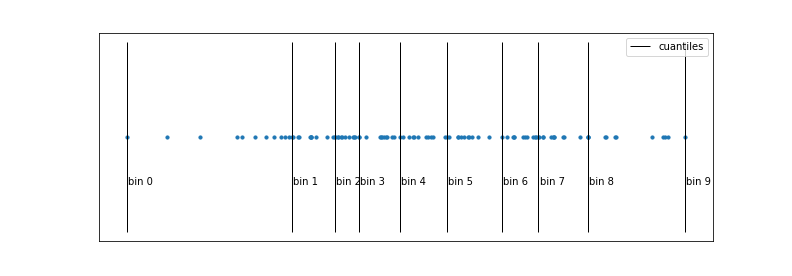
The binning strategy tries to reduce this bottleneck by speeding up the ordering of observations through a discretization of their values. Quantiles are normally used to make a homogeneous discretization in terms of the number of observations that fall into each interval. As a result of this process, the ordering is several orders of magnitude faster. The potential drawback of discretization is that some information is lost, since only the limits of each bin are considered as possible thresholds.
This is the main feature that makes the implementations of XGBoost, LightGBM, H2O and HistGradientBoosting much faster than the original scikitlearn implementation GradientBoosting.
Early stopping
One of the characteristics of Gradient Boosting models is that, with a sufficient number of weak learners, the final model tends to fit the training data perfectly, causing overfitting. This behavior implies that the analyst has to find the appropriate number of trees and, to do so, usually has to train the model with hundreds or thousands of trees until identifying the moment when overfitting begins. This is usually inefficient in terms of time, since many unnecessary trees are possibly being fitted.
To avoid this problem, most implementations include a series of strategies to stop the model fitting process from the moment it stops improving. By default, the metric used is calculated using a validation set. In scikit-learn, the stopping strategy is controlled by the arguments validation_fraction, n_iter_no_change, and tol.
Predictor Importance
While it is true that the boosting process (Gradient Boosting) improves predictive capacity compared to models based on a single tree, this has an associated cost: the interpretability of the model is reduced. Since it is a combination of multiple trees, it is not possible to obtain a simple graphical representation of the model, and it is not immediate to visually identify which predictors are more important. However, new strategies have been developed to quantify the importance of predictors that make boosting models (Gradient Boosting) a very powerful tool, not only for predicting, but also for exploratory analysis. Two of these measures are: permutation importance and node impurity.
Permutation Importance
Identifies the influence that each predictor has on a specific model evaluation metric (estimated by out-of-bag error or cross-validation). The value associated with each predictor is obtained as follows:
Create the set of trees that form the model.
Calculate a specific error metric (mse, classification error, ...). This is the reference value ($error_0$).
For each predictor $j$:
Permute the values of predictor $j$ in all the trees of the model, keeping the rest constant.
Recalculate the metric after the permutation, let's call it ($error_j$).
Calculate the increase in the metric due to the permutation of predictor $j$.
If the permuted predictor was contributing to the model, it is expected that the model's error will increase, as the information provided by that variable is lost. The percentage increase in error due to the permutation of predictor $j$ can be interpreted as the influence that $j$ has on the model. Something that often leads to confusion is the fact that this increase can be negative. If the variable does not contribute to the model, it is possible that, by reorganizing it randomly, just by chance, the model is slightly improved, so $(error_j - error_0)$ is negative. In general, it can be considered that these variables have an importance close to zero.
Although this strategy is usually the most recommended, some precautions should be taken in its interpretation. What they quantify is the influence that the predictors have on the model, not their relationship with the response variable. Why is this so important? Suppose a scenario in which this strategy is used to identify which predictors are related to a person's weight, and that two of the predictors are: body mass index (BMI) and height. Since BMI and height are highly correlated with each other (the information they provide is redundant), when one of them is permuted, the impact on the model will be minimal, since the other provides the same information. As a result, these predictors will appear as not very influential even when they are actually highly related to the response variable. One way to avoid problems of this type is, whenever predictors are excluded from a model, to check the impact it has on its predictive capacity.
Node Purity Increase
Quantifies the total increase in node purity due to splits in which the predictor participates (average of all trees). The way to calculate it is as follows: in each split of the trees, the decrease achieved in the measure used as a splitting criterion (Gini index, mse, entropy, ...) is recorded. For each of the predictors, the average decrease achieved in the set of trees that form the ensemble is calculated. The higher this average value, the greater the contribution of the predictor to the model.
Regression Example
The Boston dataset contains housing prices for the city of Boston, as well as socio-economic information about the neighborhood in which they are located. The goal is to fit a regression model that can predict the median price of a home (MEDV) based on the available variables.
Libraries
The libraries used in this example are:
# Data processing
# ==============================================================================
import numpy as np
import pandas as pd
# Plots
# ==============================================================================
import matplotlib.pyplot as plt
# Preprocessing and modeling
# ==============================================================================
import sklearn
from sklearn.ensemble import HistGradientBoostingRegressor, GradientBoostingRegressor
from sklearn.linear_model import LinearRegression
from sklearn.metrics import root_mean_squared_error
from sklearn.model_selection import cross_val_score
from sklearn.model_selection import train_test_split
from sklearn.model_selection import RepeatedKFold
from sklearn.model_selection import GridSearchCV
from sklearn.inspection import permutation_importance
import xgboost
from xgboost import XGBRegressor
import lightgbm
from lightgbm import LGBMRegressor
import multiprocessing
# Warnings configuration
# ==============================================================================
import warnings
print(f"scikit-learn version: {sklearn.__version__}")
print(f"pandas version: {pd.__version__}")
print(f"numpy version: {np.__version__}")
print(f"xgboost version: {xgboost.__version__}")
print(f"lightgbm version: {lightgbm.__version__}")
scikit-learn version: 1.7.2 pandas version: 2.3.3 numpy version: 2.2.6 xgboost version: 3.0.5 lightgbm version: 4.6.0
Data
The Boston dataset contains housing prices for the city of Boston, as well as socio-economic information about the neighborhood in which they are located. The goal is to fit a regression model that can predict the median price of a home (MEDV) based on the available variables.
Number of instances: 506
Number of attributes: 13 predictive numerical/categorical attributes.
Attribute information (in order):
- CRIM: per capita crime rate by town.
- ZN: proportion of residential land zoned for lots over 25,000 sq.ft.
- INDUS: proportion of non-retail business acres per town.
- CHAS: Charles River dummy variable (= 1 if tract bounds river; 0 otherwise).
- NOX: nitric oxides concentration (parts per 10 million).
- RM: average number of rooms per dwelling.
- AGE: proportion of owner-occupied units built prior to 1940.
- DIS: weighted distances to five Boston employment centres.
- RAD: index of accessibility to radial highways.
- TAX: full-value property-tax rate per $10,000.
- PTRATIO: pupil-teacher ratio by town.
- LSTAT: % lower status of the population.
- MEDV: Median value of owner-occupied homes in $1000's.
Missing values: None
# Data download
# ==============================================================================
url = (
'https://raw.githubusercontent.com/JoaquinAmatRodrigo/Estadistica-machine-learning-python/'
'master/data/Boston.csv'
)
data = pd.read_csv(url, sep=',')
data.head(3)
| CRIM | ZN | INDUS | CHAS | NOX | RM | AGE | DIS | RAD | TAX | PTRATIO | LSTAT | MEDV | |
|---|---|---|---|---|---|---|---|---|---|---|---|---|---|
| 0 | 0.00632 | 18.0 | 2.31 | 0 | 0.538 | 6.575 | 65.2 | 4.0900 | 1 | 296 | 15.3 | 4.98 | 24.0 |
| 1 | 0.02731 | 0.0 | 7.07 | 0 | 0.469 | 6.421 | 78.9 | 4.9671 | 2 | 242 | 17.8 | 9.14 | 21.6 |
| 2 | 0.02729 | 0.0 | 7.07 | 0 | 0.469 | 7.185 | 61.1 | 4.9671 | 2 | 242 | 17.8 | 4.03 | 34.7 |
data.info()
<class 'pandas.core.frame.DataFrame'> RangeIndex: 506 entries, 0 to 505 Data columns (total 13 columns): # Column Non-Null Count Dtype --- ------ -------------- ----- 0 CRIM 506 non-null float64 1 ZN 506 non-null float64 2 INDUS 506 non-null float64 3 CHAS 506 non-null int64 4 NOX 506 non-null float64 5 RM 506 non-null float64 6 AGE 506 non-null float64 7 DIS 506 non-null float64 8 RAD 506 non-null int64 9 TAX 506 non-null int64 10 PTRATIO 506 non-null float64 11 LSTAT 506 non-null float64 12 MEDV 506 non-null float64 dtypes: float64(10), int64(3) memory usage: 51.5 KB
Model Fitting
A model is fitted using MEDV as the response variable and all other available variables as predictors.
The HistGradientBoostingRegressor class from the sklearn.ensemble module allows training Gradient Boosting models for regression problems. The default parameters and hyperparameters are:
loss='squared_error'quantile=Nonelearning_rate=0.1max_iter=100max_leaf_nodes=31max_depth=Nonemin_samples_leaf=20l2_regularization=0.0max_bins=255categorical_features=Nonemonotonic_cst=Noneinteraction_cst=Nonewarm_start=Falseearly_stopping='auto'scoring='loss'validation_fraction=0.1n_iter_no_change=10tol=1e-07verbose=0random_state=None
A detailed description of all of them can be found at sklearn.ensemble.GradientBoostingRegressor. In practice, special attention should be paid to those that control the growth of the trees, the learning rate of the model, and those that manage early stopping to avoid overfitting:
learning_rate: reduces the contribution of each tree by multiplying its original influence by this value.max_iter: number of trees included in the model.max_depth: maximum depth that the trees can reach.min_samples_leaf: minimum number of observations that each of the child nodes must have for the split to occur. If it is a decimal value, it is interpreted as a fraction of the total training observationsceil(min_samples_split * n_samples).max_leaf_nodes: maximum number of terminal nodes that the trees can have.early_stopping: If 'auto', early stopping is activated if the sample size is greater than 10000. IfTrue, early stopping is activated; otherwise, it is deactivated.validation_fraction: proportion of data separated from the training set and used as a validation set to determine early stopping.n_iter_no_change: number of consecutive iterations in which thetolmust not be exceeded for the algorithm to stop (early stopping). If its value isNone, early stopping is deactivated.tol: minimum percentage of improvement between two consecutive iterations below which it is considered that the model has not improved.random_state: seed for the results to be reproducible. It must be an integer value.
As in any predictive study, it is not only important to fit the model, but also to quantify its ability to predict new observations. To be able to do this evaluation, the data is divided into two groups, one for training and one for testing.
# Splitting data into training and testing
# ==============================================================================
X_train, X_test, y_train, y_test = train_test_split(
data.drop(columns = "MEDV"),
data['MEDV'],
random_state = 123
)
# Model creation
# ==============================================================================
model = HistGradientBoostingRegressor(
max_iter = 10,
loss = 'squared_error',
random_state = 123
)
# Model training
# ==============================================================================
model.fit(X_train, y_train)
HistGradientBoostingRegressor(max_iter=10, random_state=123)In a Jupyter environment, please rerun this cell to show the HTML representation or trust the notebook.
On GitHub, the HTML representation is unable to render, please try loading this page with nbviewer.org.
Parameters
| loss | 'squared_error' | |
| quantile | None | |
| learning_rate | 0.1 | |
| max_iter | 10 | |
| max_leaf_nodes | 31 | |
| max_depth | None | |
| min_samples_leaf | 20 | |
| l2_regularization | 0.0 | |
| max_features | 1.0 | |
| max_bins | 255 | |
| categorical_features | 'from_dtype' | |
| monotonic_cst | None | |
| interaction_cst | None | |
| warm_start | False | |
| early_stopping | 'auto' | |
| scoring | 'loss' | |
| validation_fraction | 0.1 | |
| n_iter_no_change | 10 | |
| tol | 1e-07 | |
| verbose | 0 | |
| random_state | 123 |
Prediction and model evaluation
Once the model is trained, its predictive capacity is evaluated using the test set.
# Test error of the initial model
# ==============================================================================
predictions = model.predict(X = X_test)
rmse = root_mean_squared_error(
y_true = y_test,
y_pred = predictions,
)
print(f"The test error (rmse) is: {rmse}")
The test error (rmse) is: 5.175175457179093
Hyperparameter Optimization
The initial model has been trained using 10 trees (max_iter=10) and keeping the rest of the hyperparameters at their default values. Since they are hyperparameters, it is not possible to know in advance which is the most appropriate value; the way to identify them is by using validation strategies, for example, cross-validation.
✏️ Note
When searching for the optimal value of a hyperparameter with two different metrics, the result obtained is rarely the same. The important thing is that both metrics identify the same regions of interest.
Number of trees
In Gradient Boosting, the number of trees is a critical hyperparameter in that, as trees are added, the risk of overfitting increases.
# Validation using k-cross-validation and neg_root_mean_squared_error
# ==============================================================================
train_scores = []
cv_scores = []
# Evaluated values
max_iter_range = range(1, 500, 25)
# Loop to train a model with each value of n_estimators and extract its
# training and k-cross-validation error.
for max_iter in max_iter_range:
model = HistGradientBoostingRegressor(
max_iter = max_iter,
random_state = 123
)
# Train error
model.fit(X_train, y_train)
predictions = model.predict(X = X_train)
rmse = root_mean_squared_error(
y_true = y_train,
y_pred = predictions,
)
train_scores.append(rmse)
# Cross-validation error
scores = cross_val_score(
estimator = model,
X = X_train,
y = y_train,
scoring = 'neg_root_mean_squared_error',
cv = 5,
n_jobs = multiprocessing.cpu_count() - 1,
)
# Add the scores from cross_val_score() and convert to positive
cv_scores.append(-1*scores.mean())
# Plot with the evolution of errors
fig, ax = plt.subplots(figsize=(5, 3))
ax.plot(max_iter_range, train_scores, label="train scores")
ax.plot(max_iter_range, cv_scores, label="cv scores")
ax.plot(max_iter_range[np.argmin(cv_scores)], min(cv_scores),
marker='o', color = "red", label="min score")
ax.set_ylabel("root_mean_squared_error")
ax.set_xlabel("n_estimators")
ax.set_title("Evolution of cv-error vs number of trees")
plt.legend();
print(f"Optimal value of n_estimators: {max_iter_range[np.argmin(cv_scores)]}")
Optimal value of n_estimators: 251

The values estimated by cross-validation show that, from 50 trees onwards, the model's error stabilizes, reaching a minimum with 251 trees.
Learning rate
Along with the number of trees, the learning_rate is the most important hyperparameter in Gradient Boosting, as it is the one that allows controlling how fast the model learns and thus the risk of reaching overfitting. These two hyperparameters are interdependent; the lower the learning rate, the more trees are needed to achieve good results, but the lower the risk of overfitting.
# Validation using k-cross-validation and neg_root_mean_squared_error
# ==============================================================================
results = {}
# Evaluated values
learning_rates_grid = [0.001, 0.01, 0.1]
max_iter_grid = [10, 20, 100, 200, 300, 400, 500, 1000, 2000, 5000]
# Loop to train a model with each combination of learning_rate and n_estimator
# and extract its training and k-cross-validation error.
for learning_rate in learning_rates_grid:
train_scores = []
cv_scores = []
for n_estimator in max_iter_grid:
model = HistGradientBoostingRegressor(
max_iter = n_estimator,
learning_rate = learning_rate,
random_state = 123
)
# Train error
model.fit(X_train, y_train)
predictions = model.predict(X = X_train)
rmse = root_mean_squared_error(
y_true = y_train,
y_pred = predictions
)
train_scores.append(rmse)
# Cross-validation error
scores = cross_val_score(
estimator = model,
X = X_train,
y = y_train,
scoring = 'neg_root_mean_squared_error',
cv = 3,
n_jobs = multiprocessing.cpu_count() - 1
)
# Add the scores from cross_val_score() and convert to positive
cv_scores.append(-1*scores.mean())
results[learning_rate] = {'train_scores': train_scores, 'cv_scores': cv_scores}
# Plot with the evolution of training errors
fig, axs = plt.subplots(nrows=1, ncols=2, figsize=(9, 3))
for key, value in results.items():
axs[0].plot(max_iter_grid, value['train_scores'], label=f"Learning rate {key}")
axs[0].set_ylabel("root_mean_squared_error")
axs[0].set_xlabel("n_estimators")
axs[0].set_title("Evolution of train error vs learning rate")
axs[1].plot(max_iter_grid, value['cv_scores'], label=f"Learning rate {key}")
axs[1].set_ylabel("root_mean_squared_error")
axs[1].set_xlabel("n_estimators")
axs[1].set_title("Evolution of cv-error vs learning rate")
plt.legend();

It can be observed that the higher the value of the learning rate, the faster the model learns, but the sooner overfitting can appear. In this case, the errors estimated by cross-validation indicate that the best model is achieved with a learning rate of 0.1.
Max depth
The depth of the trees (max_depth) in Gradient Boosting models is usually a very low value, thus making each tree only able to learn a small part of the relationship between predictors and the response variable (weak learner).
# Validation using k-cross-validation and neg_root_mean_squared_error
# ==============================================================================
train_scores = []
cv_scores = []
# Evaluated values
max_depths = [1, 3, 5, 10, 20]
# Loop to train a model with each value of max_depth and extract its
# training and k-cross-validation error.
for max_depth in max_depths:
model = HistGradientBoostingRegressor(
max_iter = 25,
max_depth = max_depth,
random_state = 123
)
# Train error
model.fit(X_train, y_train)
predictions = model.predict(X = X_train)
rmse = root_mean_squared_error(
y_true = y_train,
y_pred = predictions
)
train_scores.append(rmse)
# Cross-validation error
scores = cross_val_score(
estimator = model,
X = X_train,
y = y_train,
scoring = 'neg_root_mean_squared_error',
cv = 5,
n_jobs = multiprocessing.cpu_count() - 1
)
# Add the scores from cross_val_score() and convert to positive
cv_scores.append(-1*scores.mean())
# Plot with the evolution of errors
fig, ax = plt.subplots(figsize=(5, 3))
ax.plot(max_depths, train_scores, label="train scores")
ax.plot(max_depths, cv_scores, label="cv scores")
ax.plot(max_depths[np.argmin(cv_scores)], min(cv_scores),
marker='o', color = "red", label="min score")
ax.set_ylabel("root_mean_squared_error")
ax.set_xlabel("max_depth")
ax.set_title("Evolution of cv-error vs tree depth")
plt.legend();
print(f"Optimal value of max_depth: {max_depths[np.argmin(cv_scores)]}")
Optimal value of max_depth: 5

Grid search
Although the individual analysis of hyperparameters is useful for understanding their impact on the model and identifying ranges of interest, the final search should not be done sequentially, as each hyperparameter interacts with the others. It is preferable to resort to grid search or random search to analyze various combinations of hyperparameters. More information on search strategies can be found in Machine learning with Python and Scikit-learn.
When computational resources (or time) are limited, it is advisable to follow one of the following strategies to identify the optimal hyperparameters of a Gradient Boosting model:
Fix the number of trees and optimize the learning rate.
Fix the learning rate and add as many trees as necessary, but activate early stopping to avoid overfitting.
Once the values of these hyperparameters have been identified, the rest are refined.
💡 Tip
When computational resources (or time) are limited, it is advisable to follow one of the following strategies to identify the optimal hyperparameters of a Gradient Boosting model:
Fix the number of trees and optimize the learning rate.
Fix the learning rate and add as many trees as necessary, but activate early stopping to avoid overfitting.
Grid Search based on cross-validation
In the following hyperparameter search, the strategy of not including the number of trees as a hyperparameter in the grid is used. Instead, a very high number is used by default and early stopping is activated.
In the native scikit-learn implementations (GradientBoosting and HistGradientBoosting), the validation set for early stopping is automatically extracted from the training data used in each fit, so it can be directly integrated into GridSearchCV() or RandomizedSearchCV().
# Grid of hyperparameters evaluated
# ==============================================================================
param_grid = {'loss' : ['squared_error', 'absolute_error'],
'learning_rate' : [0.001, 0.01, 0.1],
'max_depth' : [3, 5, 10, 20],
'l2_regularization': [0, 1, 10]
}
# Grid search with cross-validation
# ==============================================================================
grid = GridSearchCV(
estimator = HistGradientBoostingRegressor(
max_iter = 1000,
random_state = 123,
# Activation of early stopping
early_stopping = True,
validation_fraction = 0.1,
n_iter_no_change = 10,
tol = 1e-7,
scoring = 'loss',
),
param_grid = param_grid,
scoring = 'neg_root_mean_squared_error',
n_jobs = multiprocessing.cpu_count() - 1,
cv = RepeatedKFold(n_splits=3, n_repeats=1, random_state=123),
refit = True,
verbose = 0,
return_train_score = True
)
grid.fit(X = X_train, y = y_train)
# Results
# ==============================================================================
results = pd.DataFrame(grid.cv_results_)
results.filter(regex = '(param.*|mean_t|std_t)') \
.drop(columns = 'params') \
.sort_values('mean_test_score', ascending = False) \
.head(4)
| param_l2_regularization | param_learning_rate | param_loss | param_max_depth | mean_test_score | std_test_score | mean_train_score | std_train_score | |
|---|---|---|---|---|---|---|---|---|
| 43 | 1 | 0.1 | squared_error | 20 | -3.669431 | 0.448214 | -2.337653 | 0.595595 |
| 42 | 1 | 0.1 | squared_error | 10 | -3.669431 | 0.448214 | -2.337653 | 0.595595 |
| 17 | 0 | 0.1 | squared_error | 5 | -3.716610 | 0.384398 | -2.406267 | 0.574598 |
| 18 | 0 | 0.1 | squared_error | 10 | -3.771660 | 0.454215 | -2.478086 | 0.451284 |
# Best hyperparameters by cross-validation
# ==============================================================================
print("----------------------------------------")
print("Best hyperparameters found (cv)")
print("----------------------------------------")
print(grid.best_params_, ":", grid.best_score_, grid.scoring)
----------------------------------------
Best hyperparameters found (cv)
----------------------------------------
{'l2_regularization': 1, 'learning_rate': 0.1, 'loss': 'squared_error', 'max_depth': 10} : -3.6694305864579335 neg_root_mean_squared_error
⚠️ Warning
Although it has been indicated that n_estimator = 1000`, due to the activation of early stopping, the training may have stopped earlier.
# Number of trees in the final model (early stopping)
# ==============================================================================
print(f"Number of trees in the model: {grid.best_estimator_.n_iter_}")
Number of trees in the model: 50
Once the best hyperparameters have been identified, the model is retrained indicating the optimal values in its arguments. If refit=True is indicated in GridSearchCV(), this retraining is done automatically and the resulting model is stored in .best_estimator_.
# Test error of the final model
# ==============================================================================
final_model = grid.best_estimator_
predictions = final_model.predict(X = X_test)
rmse = root_mean_squared_error(
y_true = y_test,
y_pred = predictions
)
print(f"The test error (rmse) is: {rmse}")
The test error (rmse) is: 4.125497064570422
After optimizing the hyperparameters, the rmse error of the model is reduced from 5.2 to 4.1. The predictions of the final model are on average 4.1 units ($4100) away from the real value.
Predictor importance
HistGradientBoostingRegressor no longer incorporates predictor importance based on node purity due to evidence that this way of calculating importance is highly influenced by the number of predictors used. Instead, the use of the permutation method is recommended.
importance = permutation_importance(
estimator = final_model,
X = X_train,
y = y_train,
n_repeats = 5,
scoring = 'neg_root_mean_squared_error',
n_jobs = multiprocessing.cpu_count() - 1,
random_state = 123
)
# The results (mean and standard deviation) are stored in a dataframe
df_importance = pd.DataFrame(
{k: importance[k] for k in ['importances_mean', 'importances_std']}
)
df_importance['feature'] = X_train.columns
df_importance.sort_values('importances_mean', ascending=False)
| importances_mean | importances_std | feature | |
|---|---|---|---|
| 11 | 5.446604 | 0.288384 | LSTAT |
| 5 | 4.903891 | 0.176809 | RM |
| 7 | 0.856145 | 0.080632 | DIS |
| 4 | 0.847798 | 0.065242 | NOX |
| 0 | 0.465227 | 0.030585 | CRIM |
| 6 | 0.335038 | 0.046341 | AGE |
| 10 | 0.308566 | 0.026022 | PTRATIO |
| 9 | 0.230401 | 0.033951 | TAX |
| 2 | 0.155159 | 0.013061 | INDUS |
| 8 | 0.093236 | 0.014850 | RAD |
| 1 | 0.002374 | 0.000775 | ZN |
| 3 | 0.000000 | 0.000000 | CHAS |
# Plot
# ==============================================================================
fig, ax = plt.subplots(figsize=(5, 4))
sorted_idx = importance.importances_mean.argsort()
ax.boxplot(
importance.importances[sorted_idx].T,
vert = False,
labels = data.drop(columns = "MEDV").columns[sorted_idx]
)
ax.set_title('Predictor importance (train)')
ax.set_xlabel('Increase in error after permutation')
fig.tight_layout();

Both strategies identify LSTAT and RM as the most influential predictors, according to the training data.
XGBoost and LighGBM
XGBoost
Unlike the native scikit-learn implementations, in XGBoost and LightGBM, the validation set for early stopping is not automatically extracted. To be able to integrate early stopping with GridSearchCV() or RandomizedSearchCV() and to ensure that no observations participate in both processes, a validation set must be manually separated from the training set.
# Grid of hyperparameters evaluated
# ==============================================================================
param_grid = {'max_depth' : [3, 5, 10, 20],
'subsample' : [0.5, 1],
'learning_rate' : [0.001, 0.01, 0.1],
'booster' : ['gbtree']
}
# Create validation set
# ==============================================================================
np.random.seed(123)
validation_idx = np.random.choice(
X_train.shape[0],
size=int(X_train.shape[0]*0.1), #10% of the training data
replace=False
)
X_val = X_train.iloc[validation_idx, :].copy()
y_val = y_train.iloc[validation_idx].copy()
X_train_grid = X_train.reset_index(drop = True).drop(validation_idx, axis = 0).copy()
y_train_grid = y_train.reset_index(drop = True).drop(validation_idx, axis = 0).copy()
# XGBoost needs to pass the specific training parameters when calling
# the .fit() method
fit_params = {
"eval_set": [(X_val, y_val)],
"verbose": False
}
# Grid search with cross-validation
# ==============================================================================
grid = GridSearchCV(
estimator = XGBRegressor(
n_estimators = 1000,
early_stopping_rounds = 5,
eval_metric = "rmse",
random_state = 123
),
param_grid = param_grid,
scoring = 'neg_root_mean_squared_error',
n_jobs = multiprocessing.cpu_count() - 1,
cv = RepeatedKFold(n_splits=3, n_repeats=1, random_state=123),
refit = True,
verbose = 0,
return_train_score = True
)
grid.fit(X = X_train_grid, y = y_train_grid, **fit_params)
# Results
# ==============================================================================
results = pd.DataFrame(grid.cv_results_)
results.filter(regex = '(param.*|mean_t|std_t)') \
.drop(columns = 'params') \
.sort_values('mean_test_score', ascending = False) \
.head(4)
| param_booster | param_learning_rate | param_max_depth | param_subsample | mean_test_score | std_test_score | mean_train_score | std_train_score | |
|---|---|---|---|---|---|---|---|---|
| 18 | gbtree | 0.10 | 5 | 0.5 | -3.780975 | 0.601978 | -1.222699 | 0.670224 |
| 22 | gbtree | 0.10 | 20 | 0.5 | -3.814522 | 0.676036 | -1.098650 | 0.380221 |
| 20 | gbtree | 0.10 | 10 | 0.5 | -3.889702 | 0.649555 | -1.098182 | 0.620475 |
| 14 | gbtree | 0.01 | 20 | 0.5 | -3.893593 | 0.603064 | -1.705033 | 0.405872 |
# Best hyperparameters by cross-validation
# ==============================================================================
print("----------------------------------------")
print("Best hyperparameters found (cv)")
print("----------------------------------------")
print(grid.best_params_, ":", grid.best_score_, grid.scoring)
# Number of trees in the final model (early stopping)
# ==============================================================================
n_trees_included = len(grid.best_estimator_.get_booster().get_dump())
print(f"Number of trees included in the model: {n_trees_included}")
----------------------------------------
Best hyperparameters found (cv)
----------------------------------------
{'booster': 'gbtree', 'learning_rate': 0.1, 'max_depth': 5, 'subsample': 0.5} : -3.7809748896923665 neg_root_mean_squared_error
Number of trees included in the model: 34
# Test error of the final model
# ==============================================================================
final_model = grid.best_estimator_
predictions = final_model.predict(X_test)
rmse = root_mean_squared_error(
y_true = y_test,
y_pred = predictions
)
print(f"The test error (rmse) is: {rmse}")
The test error (rmse) is: 3.7360376054022693
LightGBM
For this example, the number of trees is included in the search instead of activating early stopping.
# Grid of hyperparameters evaluated
# =================================================================-1,=============
param_grid = {'n_estimators' : [100, 500, 1000],
'max_depth' : [3, 5, 10, 20],
'subsample' : [0.5, 1],
'learning_rate' : [0.001, 0.01, 0.1],
'boosting_type' : ['gbdt']
}
# Grid search with cross-validation
# ==============================================================================
grid = GridSearchCV(
estimator = LGBMRegressor(random_state=123, verbose=-1),
param_grid = param_grid,
scoring = 'neg_root_mean_squared_error',
n_jobs = multiprocessing.cpu_count() - 1,
cv = RepeatedKFold(n_splits=3, n_repeats=1, random_state=123),
refit = True,
verbose = 0,
return_train_score = True
)
grid.fit(X = X_train_grid, y = y_train_grid)
# Results
# ==============================================================================
results = pd.DataFrame(grid.cv_results_)
results.filter(regex = '(param.*|mean_t|std_t)') \
.drop(columns = 'params') \
.sort_values('mean_test_score', ascending = False) \
.head(4)
| param_boosting_type | param_learning_rate | param_max_depth | param_n_estimators | param_subsample | mean_test_score | std_test_score | mean_train_score | std_train_score | |
|---|---|---|---|---|---|---|---|---|---|
| 50 | gbdt | 0.1 | 3 | 500 | 0.5 | -3.803656 | 0.772055 | -1.071614 | 0.104883 |
| 51 | gbdt | 0.1 | 3 | 500 | 1.0 | -3.803656 | 0.772055 | -1.071614 | 0.104883 |
| 60 | gbdt | 0.1 | 10 | 100 | 0.5 | -3.805746 | 0.764872 | -1.773668 | 0.183944 |
| 61 | gbdt | 0.1 | 10 | 100 | 1.0 | -3.805746 | 0.764872 | -1.773668 | 0.183944 |
# Best hyperparameters by cross-validation
# ==============================================================================
print("----------------------------------------")
print("Best hyperparameters found (cv)")
print("----------------------------------------")
print(grid.best_params_, ":", grid.best_score_, grid.scoring)
----------------------------------------
Best hyperparameters found (cv)
----------------------------------------
{'boosting_type': 'gbdt', 'learning_rate': 0.1, 'max_depth': 3, 'n_estimators': 500, 'subsample': 0.5} : -3.8036560847224155 neg_root_mean_squared_error
# Test error of the final model
# ==============================================================================
final_model = grid.best_estimator_
predictions = final_model.predict(X = X_test,)
rmse = root_mean_squared_error(
y_true = y_test,
y_pred = predictions
)
print(f"The test error (rmse) is: {rmse}")
The test error (rmse) is: 4.1326656546767015
Classification Example
Libraries
The libraries used in this document are:
# Data processing
# ==============================================================================
import numpy as np
import pandas as pd
import statsmodels.api as sm
# Plots
# ==============================================================================
import matplotlib.pyplot as plt
# Preprocessing and modeling
# ==============================================================================
from sklearn.ensemble import HistGradientBoostingClassifier
from sklearn.metrics import accuracy_score
from sklearn.metrics import confusion_matrix
from sklearn.metrics import ConfusionMatrixDisplay
from sklearn.compose import make_column_transformer
from sklearn.preprocessing import OrdinalEncoder
from sklearn.model_selection import cross_val_score
from sklearn.model_selection import train_test_split
from sklearn.model_selection import RepeatedKFold
from sklearn.model_selection import GridSearchCV
from sklearn.inspection import permutation_importance
import xgboost
from xgboost import XGBClassifier
import lightgbm
from lightgbm import LGBMClassifier
import multiprocessing
# Warnings configuration
# ==============================================================================
import warnings
print(f"scikit-learn version: {sklearn.__version__}")
print(f"pandas version: {pd.__version__}")
print(f"numpy version: {np.__version__}")
print(f"xgboost version: {xgboost.__version__}")
print(f"lightgbm version: {lightgbm.__version__}")
scikit-learn version: 1.7.2 pandas version: 2.3.3 numpy version: 2.2.6 xgboost version: 3.0.5 lightgbm version: 4.6.0
Data
The Carseats dataset, originally from the R package ISLR and accessible in Python through statsmodels.datasets.get_rdataset, contains information about the sale of child car seats in 400 different stores. For each of the 400 stores, 11 variables have been recorded. The goal is to generate a classification model that can predict whether a store has high sales (Sales > 8) or low sales (Sales <= 8) based on all available variables.
✏️ Note
List of all available datasets in Rdatasets
# Data loading
# ==============================================================================
carseats = sm.datasets.get_rdataset("Carseats", "ISLR")
data = carseats.data
data.head(3)
| Sales | CompPrice | Income | Advertising | Population | Price | ShelveLoc | Age | Education | Urban | US | |
|---|---|---|---|---|---|---|---|---|---|---|---|
| 0 | 9.50 | 138 | 73 | 11 | 276 | 120 | Bad | 42 | 17 | Yes | Yes |
| 1 | 11.22 | 111 | 48 | 16 | 260 | 83 | Good | 65 | 10 | Yes | Yes |
| 2 | 10.06 | 113 | 35 | 10 | 269 | 80 | Medium | 59 | 12 | Yes | Yes |
Since Sales is a continuous variable and the objective of the study is to classify stores based on whether they sell a lot or a little, a new binary variable (0, 1) called high_sales is created.
data['high_sales'] = np.where(data.Sales > 8, 0, 1)
# Once the new response variable is created, the original one is discarded
data = data.drop(columns = 'Sales')
Model fitting and hyperparameter optimization
A classification model is fitted using high_sales as the response variable and all available variables as predictors.
✏️ Note
Unlike the previous example, this data includes categorical variables. Although all the libraries used in this document are capable of handling categorical variables natively, in some models or implementations it might be necessary to apply the one-hot-encoding technique. The section titled Categorical Variables provides a detailed analysis of the use of these variables with each of the libraries.
# Splitting data into train and test
# ==============================================================================
X_train, X_test, y_train, y_test = train_test_split(
data.drop(columns = 'high_sales'),
data['high_sales'],
random_state = 123
)
# Ordinal encoding of categorical variables
# ==============================================================================
# The names of the categorical columns are identified
cat_cols = X_train.select_dtypes(include=['object', 'category']).columns.to_list()
# HistGradientBoostingClassifier requires that category values be encoded
# in [0, n_unique_categories - 1], so an OrdinalEncoder is used to
# preprocess the data. Missing values are encoded as -1. If a new
# category is found in the test set, it is encoded as -1.
cat_cols = X_train.select_dtypes(exclude=[np.number]).columns.tolist()
preprocessor = make_column_transformer(
(
OrdinalEncoder(
dtype=int,
handle_unknown="use_encoded_value",
unknown_value=-1,
encoded_missing_value=-1
),
cat_cols
),
remainder="passthrough",
verbose_feature_names_out=False,
).set_output(transform="pandas")
# Once the ColumnTransformer object has been defined, with the fit() method
# the transformations are learned with the training data and applied to
# the two sets with transform(). Both operations at the same time with fit_transform().
X_train_prep = preprocessor.fit_transform(X_train)
X_test_prep = preprocessor.transform(X_test)
X_train_prep.info()
<class 'pandas.core.frame.DataFrame'> Index: 300 entries, 170 to 365 Data columns (total 10 columns): # Column Non-Null Count Dtype --- ------ -------------- ----- 0 ShelveLoc 300 non-null int64 1 Urban 300 non-null int64 2 US 300 non-null int64 3 CompPrice 300 non-null int64 4 Income 300 non-null int64 5 Advertising 300 non-null int64 6 Population 300 non-null int64 7 Price 300 non-null int64 8 Age 300 non-null int64 9 Education 300 non-null int64 dtypes: int64(10) memory usage: 25.8 KB
Although HistGradientBoostingClassifier has default values for its hyperparameters, it is not possible to know in advance if these are the most appropriate; the way to identify them is by using validation strategies, for example, cross-validation. It should be noted that when searching for the optimal value of a hyperparameter with two different metrics, the result obtained is rarely the same. The important thing is that both metrics identify the same regions of interest.
Although the individual analysis of hyperparameters is useful for understanding their impact on the model and identifying ranges of interest, the final search should not be done sequentially, as each hyperparameter interacts with the others. It is preferable to resort to grid search or random search to analyze various combinations of hyperparameters. More information on search strategies can be found in Machine learning with Python and Scikit-learn.
Grid Search based on cross-validation
# Grid of hyperparameters evaluated
# ==============================================================================
param_grid = {
'max_iter' : [50, 100, 500, 1000],
'max_depth' : [3, 5, 10, 20],
'learning_rate' : [0.001, 0.01, 0.1]
}
# Grid search with cross-validation
# ==============================================================================
grid = GridSearchCV(
estimator = HistGradientBoostingClassifier(random_state=123, categorical_features=cat_cols),
param_grid = param_grid,
scoring = 'accuracy',
n_jobs = multiprocessing.cpu_count() - 1,
cv = RepeatedKFold(n_splits=3, n_repeats=1, random_state=123),
refit = True,
verbose = 0,
return_train_score = True
)
grid.fit(X = X_train_prep, y = y_train)
# Results
# ==============================================================================
results = pd.DataFrame(grid.cv_results_)
results.filter(regex = '(param*|mean_t|std_t)') \
.drop(columns = 'params') \
.sort_values('mean_test_score', ascending = False) \
.head(4)
| param_learning_rate | param_max_depth | param_max_iter | mean_test_score | std_test_score | mean_train_score | std_train_score | |
|---|---|---|---|---|---|---|---|
| 38 | 0.1 | 5 | 500 | 0.843333 | 0.054365 | 1.0 | 0.0 |
| 34 | 0.1 | 3 | 500 | 0.836667 | 0.061824 | 1.0 | 0.0 |
| 39 | 0.1 | 5 | 1000 | 0.836667 | 0.049889 | 1.0 | 0.0 |
| 43 | 0.1 | 10 | 1000 | 0.833333 | 0.062361 | 1.0 | 0.0 |
# Best hyperparameters by cross-validation
# ==============================================================================
print("----------------------------------------")
print("Best hyperparameters found (cv)")
print("----------------------------------------")
print(grid.best_params_, ":", grid.best_score_, grid.scoring)
----------------------------------------
Best hyperparameters found (cv)
----------------------------------------
{'learning_rate': 0.1, 'max_depth': 5, 'max_iter': 500} : 0.8433333333333333 accuracy
Once the best hyperparameters have been identified, the model is retrained indicating the optimal values in its arguments. If refit=True is indicated in GridSearchCV(), this retraining is done automatically and
the resulting model is stored in .best_estimator_.
final_model = grid.best_estimator_
final_model
HistGradientBoostingClassifier(categorical_features=['ShelveLoc', 'Urban',
'US'],
max_depth=5, max_iter=500, random_state=123)In a Jupyter environment, please rerun this cell to show the HTML representation or trust the notebook. On GitHub, the HTML representation is unable to render, please try loading this page with nbviewer.org.
Parameters
| loss | 'log_loss' | |
| learning_rate | 0.1 | |
| max_iter | 500 | |
| max_leaf_nodes | 31 | |
| max_depth | 5 | |
| min_samples_leaf | 20 | |
| l2_regularization | 0.0 | |
| max_features | 1.0 | |
| max_bins | 255 | |
| categorical_features | ['ShelveLoc', 'Urban', ...] | |
| monotonic_cst | None | |
| interaction_cst | None | |
| warm_start | False | |
| early_stopping | 'auto' | |
| scoring | 'loss' | |
| validation_fraction | 0.1 | |
| n_iter_no_change | 10 | |
| tol | 1e-07 | |
| verbose | 0 | |
| random_state | 123 | |
| class_weight | None |
Prediction and model evaluation
Finally, the predictive capacity of the final model is evaluated using the test set.
# Test error of the final model
# ==============================================================================
predictions = final_model.predict(X = X_test_prep)
predictions[:10]
array([0, 1, 0, 0, 0, 0, 1, 1, 1, 1])
confusion_mat = confusion_matrix(
y_true = y_test,
y_pred = predictions
)
accuracy = accuracy_score(
y_true = y_test,
y_pred = predictions,
normalize = True
)
print("Confusion matrix")
print("-------------------")
print(confusion_mat)
print("")
print(f"The test accuracy is: {100 * accuracy} %")
fig, ax = plt.subplots(figsize=(3, 3))
ConfusionMatrixDisplay(confusion_mat).plot(ax=ax);
Confusion matrix ------------------- [[38 12] [ 5 45]] The test accuracy is: 83.0 %

After optimizing the hyperparameters, an accuracy of 83% is achieved.
Probability Prediction
Most implementations of Gradient Boosting Trees, including that of scikit-learn, allow for the prediction of probabilities when dealing with classification problems. It is important to understand how these values are calculated to interpret and use them correctly.
In the previous example, applying .predict() returns $1$ (high sales) or $0$ (low sales) for each test observation. However, no information is available about the confidence with which the model makes this assignment. With .predict_proba(), instead of a classification, the probability with which the model considers that each observation may belong to each of the classes is obtained.
# Probability prediction
# ==============================================================================
predictions = final_model.predict_proba(X = X_test_prep)
predictions[:5, :]
array([[8.35357869e-01, 1.64642131e-01],
[2.15360382e-01, 7.84639618e-01],
[9.99999727e-01, 2.73092904e-07],
[8.22826079e-01, 1.77173921e-01],
[9.99996651e-01, 3.34906400e-06]])
The result of .predict_proba() is an array with one row per observation and as many columns as there are classes in the response variable. The value of the first column corresponds to the probability, according to the model, that the observation belongs to class 0, and so on. The probability value shown for each prediction corresponds to the fraction of observations of each class in the terminal nodes that the predicted observation has reached in the set of trees.
By default, .predict() assigns each new observation to the class with the highest probability (in case of a tie, it is assigned randomly). However, this may not be the desired behavior in all cases.
# Classification using the class with the highest probability
# ==============================================================================
df_predictions = pd.DataFrame(data=predictions, columns=['0', '1'])
df_predictions['default_classification_0.5'] = np.where(df_predictions['0'] > df_predictions['1'], 0, 1)
df_predictions.head(3)
| 0 | 1 | default_classification_0.5 | |
|---|---|---|---|
| 0 | 0.835358 | 1.646421e-01 | 0 |
| 1 | 0.215360 | 7.846396e-01 | 1 |
| 2 | 1.000000 | 2.730929e-07 | 0 |
Suppose the following scenario: the Christmas campaign is approaching and the owners of the chain want to double the stock of items in those stores that are predicted to have high sales. Since transporting this material to the stores involves a high cost, the director wants to limit this strategy only to stores for which there is a high degree of certainty that they will achieve high sales.
If probabilities are available, a specific cutoff point can be established, for example, considering only as class $1$ (high sales) those stores whose prediction for this class is greater than 0.9 (90%). In this way, the final classification is better adjusted to the needs of the use case.
# Final classification using a threshold of 0.8 for class 1.
# ==============================================================================
df_predictions['custom_classification_0.8'] = np.where(df_predictions['1'] > 0.9, 1, 0)
df_predictions[df_predictions['custom_classification_0.8']!=df_predictions['default_classification_0.5']] \
.head(3)
| 0 | 1 | default_classification_0.5 | custom_classification_0.8 | |
|---|---|---|---|---|
| 1 | 0.215360 | 0.784640 | 1 | 0 |
| 33 | 0.227356 | 0.772644 | 1 | 0 |
| 95 | 0.117894 | 0.882106 | 1 | 0 |
To what extent should these probabilities be trusted?
It is very important to consider the difference between the model's "view" of the world and the real world. All a model knows about the real world is what it has been able to learn from the training data and, therefore, it has a limited "view". For example, suppose that, in the training data, all stores in an urban area Urban='Yes' have high sales regardless of the value of the other predictors. When the model tries to predict a new observation, if it is in an urban area, it will classify the store as high sales with 100% certainty. However, this does not mean that it is unequivocally true; there could be stores in urban areas that do not have high sales but, since they are not present in the training data, the model does not consider this possibility.
Taking all this into account, the probabilities generated by the model must be considered as the certainty that it has, from its limited view, when making predictions. But not as the probability in the real world that it is so.
Predictor importance
Permutation importance
importance = permutation_importance(
estimator = final_model,
X = X_train_prep,
y = y_train,
n_repeats = 5,
scoring = 'accuracy',
n_jobs = multiprocessing.cpu_count() - 1,
random_state = 123
)
# The results (mean and standard deviation) are stored in a dataframe
df_importance = pd.DataFrame(
{k: importance[k] for k in ['importances_mean', 'importances_std']}
)
df_importance['feature'] = X_train_prep.columns
df_importance.sort_values('importances_mean', ascending=False)
| importances_mean | importances_std | feature | |
|---|---|---|---|
| 7 | 0.498954 | 0.019444 | Price |
| 0 | 0.454362 | 0.014888 | ShelveLoc |
| 3 | 0.364298 | 0.024908 | CompPrice |
| 5 | 0.297150 | 0.019205 | Advertising |
| 8 | 0.210673 | 0.016837 | Age |
| 4 | 0.172179 | 0.018822 | Income |
| 6 | 0.050971 | 0.027116 | Population |
| 1 | 0.000000 | 0.000000 | Urban |
| 2 | 0.000000 | 0.000000 | US |
| 9 | 0.000000 | 0.000000 | Education |
# Plot
# ==============================================================================
fig, ax = plt.subplots(figsize=(3.5, 4))
df_importance = df_importance.sort_values('importances_mean', ascending=True)
ax.barh(
df_importance['feature'],
df_importance['importances_mean'],
xerr=df_importance['importances_std'],
align='center',
alpha=0
)
ax.plot(
df_importance['importances_mean'],
df_importance['feature'],
marker="D",
linestyle="",
alpha=0.8,
color="r"
)
ax.set_title('Predictor importance (train)')
ax.set_xlabel('Increase in error after permutation');

According to the training data, Price and ShelveLoc are identified as the most influential predictors, closely followed by CompPrice and Advertising.
Categorical Variables
In the field of machine learning, categorical variables play a fundamental role in determining the predictive capacity of a model. Categorical variables are those that can take a limited number of values, such as color, gender, or location. While these variables can provide useful information about the patterns and relationships in the data, they present unique challenges.
One of these challenges is the need to convert categorical values into numerical values that can be processed by machine learning algorithms. Another challenge arises when dealing with infrequent categories, which can lead to biased models. If a categorical variable has a large number of categories, but some of them appear infrequently in the data, the model may not be able to learn from them, leading to biased predictions and inaccurate results. Despite these difficulties, categorical variables remain an essential component in many use cases. When properly encoded and handled, they can provide very useful information to achieve better predictions.
Some models such as XGBoost, LightGBM, CatBoost, and HistGradientBoosting, are able to handle categorical predictors natively, but they assume that the categories are integers starting from 0 up to the number of categories [0, 1, ..., n_categories-1]. In practice, categorical variables are not usually encoded as numbers, but with character strings (strings), so an intermediate transformation step is necessary. There are two options:
Convert the columns with categorical variables to the
pandas.categorytype. In pandas, the data structure of acategorytype column consists of an array of categories and an array of integer values (codes) that point to the actual value in the category array. That is, internally it is a numerical array with a mapping that relates each value to a category. The models are able to automatically identify thecategorytype columns and access their internal codes. This approach is applicable to XGBoost, LightGBM, and CatBoost.Preprocess the categorical columns with an
OrdinalEncoderto transform their values into integers and explicitly indicate that the columns should be treated as categorical. If this last step is not performed, the models will treat the variables as if they were numerical.
⚠️ Warning
When deploying models in production, it is strongly recommended to avoid using automatic detection based on Pandas category type columns. Although Pandas provides an internal encoding for these columns, it is not consistent across different datasets and can vary depending on the categories present in each one. Therefore, it is crucial to be aware of this issue and take appropriate measures to ensure consistency in the encoding of categorical variables when deploying models in production. More details on this issue can be found in this github issue and on stackoverflow.
✏️ Note
The following examples are intended to show how to incorporate categorical variables into the models; the rest of the settings are left at their default values.
LightGBM
LightGBM allows both automatic detection based on the column type and indicating which columns should be treated as categories (as long as they have been previously encoded as integers). The two approaches are shown below.
Encode categories as integers and explicitly specify the names of the categorical variables (recommended)
# Data loading
# ==============================================================================
carseats = sm.datasets.get_rdataset("Carseats", "ISLR")
data = carseats.data
data['high_sales'] = np.where(data.Sales > 8, 0, 1)
# Once the new response variable is created, the original one is discarded
data = data.drop(columns = 'Sales')
# Splitting data into train and test
# ==============================================================================
X_train, X_test, y_train, y_test = train_test_split(
data.drop(columns = 'high_sales'),
data['high_sales'],
random_state = 123
)
# Ordinal encoding of categorical variables
# ==============================================================================
# An OrdinalEncoder is used to preprocess the data. Missing values are encoded
# as -1. If a new category is found in the test set, it is encoded as -1.
cat_cols = X_train.select_dtypes(exclude=[np.number]).columns.tolist()
preprocessor = make_column_transformer(
(
OrdinalEncoder(
dtype=int,
handle_unknown="use_encoded_value",
unknown_value=-1,
encoded_missing_value=-1
),
cat_cols
),
remainder="passthrough",
verbose_feature_names_out=False,
).set_output(transform="pandas")
# Once the ColumnTransformer object has been defined, with the fit() method
# the transformations are learned with the training data and applied to
# the two sets with transform(). Both operations at the same time with fit_transform().
X_train_prep = preprocessor.fit_transform(X_train)
X_test_prep = preprocessor.transform(X_test)
# Model training
# ==============================================================================
model = LGBMClassifier(
n_estimators = 100,
random_state = 123,
verbose = -1
)
# In the LGBMRegressor and LGBMClassifier models, the categorical_feature argument
# is specified in the fit method and not during its initialization.
model.fit(X = X_train_prep, y = y_train, categorical_feature=cat_cols)
LGBMClassifier(random_state=123, verbose=-1)In a Jupyter environment, please rerun this cell to show the HTML representation or trust the notebook.
On GitHub, the HTML representation is unable to render, please try loading this page with nbviewer.org.
Parameters
| boosting_type | 'gbdt' | |
| num_leaves | 31 | |
| max_depth | -1 | |
| learning_rate | 0.1 | |
| n_estimators | 100 | |
| subsample_for_bin | 200000 | |
| objective | None | |
| class_weight | None | |
| min_split_gain | 0.0 | |
| min_child_weight | 0.001 | |
| min_child_samples | 20 | |
| subsample | 1.0 | |
| subsample_freq | 0 | |
| colsample_bytree | 1.0 | |
| reg_alpha | 0.0 | |
| reg_lambda | 0.0 | |
| random_state | 123 | |
| n_jobs | None | |
| importance_type | 'split' | |
| verbose | -1 |
The UserWarning indicates that categorical predictors have been included. This warning can be suppressed using warnings.filterwarnings('ignore') and re-enabled with warnings.filterwarnings('default') or warnings.resetwarnings().
# Predictions
# ==============================================================================
predictions = model.predict(X = X_test_prep)
predictions
array([0, 0, 0, 0, 0, 1, 1, 1, 1, 1, 1, 1, 1, 1, 0, 0, 0, 1, 1, 1, 1, 1,
1, 0, 1, 1, 0, 1, 0, 1, 0, 1, 1, 0, 0, 1, 1, 1, 1, 0, 1, 1, 1, 0,
1, 0, 0, 0, 1, 1, 0, 1, 1, 0, 1, 1, 0, 1, 1, 0, 1, 1, 1, 0, 0, 1,
0, 0, 0, 0, 1, 1, 0, 1, 0, 1, 1, 0, 1, 1, 1, 0, 1, 0, 0, 0, 1, 0,
1, 1, 0, 1, 0, 1, 1, 1, 1, 1, 0, 1])
Automatic detection of categorical variables
# Data loading
# ==============================================================================
carseats = sm.datasets.get_rdataset("Carseats", "ISLR")
data = carseats.data
data['high_sales'] = np.where(data.Sales > 8, 0, 1)
# Once the new response variable is created, the original one is discarded
data = data.drop(columns = 'Sales')
# Convert non-numeric variables to category type
# ==============================================================================
cat_cols = X_train.select_dtypes(exclude=[np.number]).columns.tolist()
data[cat_cols] = data[cat_cols].astype('category')
# Splitting data into train and test
# ==============================================================================
X_train, X_test, y_train, y_test = train_test_split(
data.drop(columns = 'high_sales'),
data['high_sales'],
random_state = 123
)
# Model training
# ==============================================================================
model = LGBMClassifier(
n_estimators = 100,
random_state = 123,
verbose = -1
)
# In the LGBMRegressor and LGBMClassifier models, the categorical_feature argument
# is specified in the fit method and not during its initialization.
model.fit(X = X_train, y = y_train, categorical_feature='auto')
LGBMClassifier(random_state=123, verbose=-1)In a Jupyter environment, please rerun this cell to show the HTML representation or trust the notebook.
On GitHub, the HTML representation is unable to render, please try loading this page with nbviewer.org.
Parameters
| boosting_type | 'gbdt' | |
| num_leaves | 31 | |
| max_depth | -1 | |
| learning_rate | 0.1 | |
| n_estimators | 100 | |
| subsample_for_bin | 200000 | |
| objective | None | |
| class_weight | None | |
| min_split_gain | 0.0 | |
| min_child_weight | 0.001 | |
| min_child_samples | 20 | |
| subsample | 1.0 | |
| subsample_freq | 0 | |
| colsample_bytree | 1.0 | |
| reg_alpha | 0.0 | |
| reg_lambda | 0.0 | |
| random_state | 123 | |
| n_jobs | None | |
| importance_type | 'split' | |
| verbose | -1 |
# Predictions
# ==============================================================================
predictions = model.predict(X = X_test)
predictions
array([0, 0, 0, 0, 0, 1, 1, 1, 1, 1, 1, 1, 1, 1, 0, 0, 0, 1, 1, 1, 1, 1,
1, 0, 1, 1, 0, 1, 0, 1, 0, 1, 1, 0, 0, 1, 1, 1, 1, 0, 1, 1, 1, 0,
1, 0, 0, 0, 1, 1, 0, 1, 1, 0, 1, 1, 0, 1, 1, 0, 1, 1, 1, 0, 0, 1,
0, 0, 0, 0, 1, 1, 0, 1, 0, 1, 1, 0, 1, 1, 1, 0, 1, 0, 0, 0, 1, 0,
1, 1, 0, 1, 0, 1, 1, 1, 1, 1, 0, 1])
Scikit-learn HistogramGradientBoosting
Scikit-learn does not include automatic detection of categorical variables based on column type. Instead, it is necessary to indicate which columns are categorical during the model instantiation using the categorical_feature argument. In addition, the values of these columns must be encoded as integers.
# Data loading
# ==============================================================================
carseats = sm.datasets.get_rdataset("Carseats", "ISLR")
data = carseats.data
data['high_sales'] = np.where(data.Sales > 8, 0, 1)
# Once the new response variable is created, the original one is discarded
data = data.drop(columns = 'Sales')
# Splitting data into train and test
# ==============================================================================
X_train, X_test, y_train, y_test = train_test_split(
data.drop(columns = 'high_sales'),
data['high_sales'],
random_state = 123
)
# Ordinal encoding of categorical variables
# ==============================================================================
# OrdinalEncoder to preprocess the data. Missing values are encoded
# as -1. If a new category is found in the test set, it is encoded
# as -1.
cat_cols = X_train.select_dtypes(exclude=[np.number]).columns.tolist()
preprocessor = make_column_transformer(
(
OrdinalEncoder(
dtype=int,
handle_unknown="use_encoded_value",
unknown_value=-1,
encoded_missing_value=-1
),
cat_cols
),
remainder="passthrough",
verbose_feature_names_out=False,
).set_output(transform="pandas")
# Once the ColumnTransformer object has been defined, with the fit() method
# the transformations are learned with the training data and applied to
# the two sets with transform(). Both operations at the same time with fit_transform().
X_train_prep = preprocessor.fit_transform(X_train)
X_test_prep = preprocessor.transform(X_test)
# Model training
# ==============================================================================
model = HistGradientBoostingClassifier(
max_iter = 100,
categorical_features = cat_cols,
random_state = 123
)
model.fit(X = X_train_prep, y = y_train)
HistGradientBoostingClassifier(categorical_features=['ShelveLoc', 'Urban',
'US'],
random_state=123)In a Jupyter environment, please rerun this cell to show the HTML representation or trust the notebook. On GitHub, the HTML representation is unable to render, please try loading this page with nbviewer.org.
Parameters
| loss | 'log_loss' | |
| learning_rate | 0.1 | |
| max_iter | 100 | |
| max_leaf_nodes | 31 | |
| max_depth | None | |
| min_samples_leaf | 20 | |
| l2_regularization | 0.0 | |
| max_features | 1.0 | |
| max_bins | 255 | |
| categorical_features | ['ShelveLoc', 'Urban', ...] | |
| monotonic_cst | None | |
| interaction_cst | None | |
| warm_start | False | |
| early_stopping | 'auto' | |
| scoring | 'loss' | |
| validation_fraction | 0.1 | |
| n_iter_no_change | 10 | |
| tol | 1e-07 | |
| verbose | 0 | |
| random_state | 123 | |
| class_weight | None |
# Predictions
# ==============================================================================
predictions = model.predict(X = X_test_prep)
predictions
array([1, 0, 0, 0, 0, 0, 1, 1, 1, 1, 1, 1, 1, 1, 0, 0, 0, 1, 1, 1, 1, 1,
1, 0, 1, 1, 0, 1, 0, 1, 0, 1, 1, 1, 0, 1, 1, 1, 1, 0, 1, 1, 1, 0,
1, 0, 0, 0, 1, 1, 0, 1, 1, 0, 1, 0, 0, 1, 1, 0, 1, 1, 1, 1, 0, 0,
0, 0, 0, 0, 1, 1, 0, 1, 0, 1, 1, 0, 1, 1, 0, 0, 1, 0, 0, 0, 1, 0,
1, 1, 0, 1, 0, 0, 1, 1, 1, 1, 0, 1])
XGBoost
XGBoost allows both automatic detection based on column type and indicating which columns should be treated as categories (as long as they have been previously encoded as integers). Unlike LightGBM or scikit-learn, XGBoost does not provide an option to indicate the names of the categorical variables. Instead, the variable types are specified by passing a list to the feature_types argument, where 'c' denotes categorical variables and 'q' numerical. In addition, the enable_categorical argument must be True and tree_method 'hist'.
Encode categories as integers and explicitly specify the categorical variables (recommended)
# Data loading
# ==============================================================================
carseats = sm.datasets.get_rdataset("Carseats", "ISLR")
data = carseats.data
data['high_sales'] = np.where(data.Sales > 8, 0, 1)
# Once the new response variable is created, the original one is discarded
data = data.drop(columns = 'Sales')
# Splitting data into train and test
# ==============================================================================
X_train, X_test, y_train, y_test = train_test_split(
data.drop(columns = 'high_sales'),
data['high_sales'],
random_state = 123
)
# Ordinal encoding of categorical variables
# ==============================================================================
# An OrdinalEncoder is used to preprocess the data. Missing values are
# encoded as -1. If a new category is found in the test set, it is encoded
# as -1.
cat_cols = X_train.select_dtypes(exclude=[np.number]).columns.tolist()
preprocessor = make_column_transformer(
(
OrdinalEncoder(
dtype=int,
handle_unknown="use_encoded_value",
unknown_value=-1,
encoded_missing_value=-1
),
cat_cols
),
remainder="passthrough",
verbose_feature_names_out=False,
).set_output(transform="pandas")
# Once the ColumnTransformer object has been defined, with the fit() method
# the transformations are learned with the training data and applied to
# the two sets with transform(). Both operations at the same time with fit_transform().
X_train_prep = preprocessor.fit_transform(X_train)
X_test_prep = preprocessor.transform(X_test)
# A list is created to identify if each column is categorical ('c') or numerical ('q')
feature_types = ['c' if col in cat_cols else 'q' for col in X_train_prep.columns]
feature_types
['c', 'c', 'c', 'q', 'q', 'q', 'q', 'q', 'q', 'q']
# Model training
# ==============================================================================
model = XGBClassifier(
n_estimators = 100,
tree_method='hist',
enable_categorical=True,
feature_types=feature_types,
random_state = 123
)
model.fit(X = X_train_prep, y = y_train)
XGBClassifier(base_score=None, booster=None, callbacks=None,
colsample_bylevel=None, colsample_bynode=None,
colsample_bytree=None, device=None, early_stopping_rounds=None,
enable_categorical=True, eval_metric=None,
feature_types=['c', 'c', 'c', 'q', 'q', 'q', 'q', 'q', 'q', 'q'],
feature_weights=None, gamma=None, grow_policy=None,
importance_type=None, interaction_constraints=None,
learning_rate=None, max_bin=None, max_cat_threshold=None,
max_cat_to_onehot=None, max_delta_step=None, max_depth=None,
max_leaves=None, min_child_weight=None, missing=nan,
monotone_constraints=None, multi_strategy=None, n_estimators=100,
n_jobs=None, num_parallel_tree=None, ...)In a Jupyter environment, please rerun this cell to show the HTML representation or trust the notebook. On GitHub, the HTML representation is unable to render, please try loading this page with nbviewer.org.
Parameters
| objective | 'binary:logistic' | |
| base_score | None | |
| booster | None | |
| callbacks | None | |
| colsample_bylevel | None | |
| colsample_bynode | None | |
| colsample_bytree | None | |
| device | None | |
| early_stopping_rounds | None | |
| enable_categorical | True | |
| eval_metric | None | |
| feature_types | ['c', 'c', ...] | |
| feature_weights | None | |
| gamma | None | |
| grow_policy | None | |
| importance_type | None | |
| interaction_constraints | None | |
| learning_rate | None | |
| max_bin | None | |
| max_cat_threshold | None | |
| max_cat_to_onehot | None | |
| max_delta_step | None | |
| max_depth | None | |
| max_leaves | None | |
| min_child_weight | None | |
| missing | nan | |
| monotone_constraints | None | |
| multi_strategy | None | |
| n_estimators | 100 | |
| n_jobs | None | |
| num_parallel_tree | None | |
| random_state | 123 | |
| reg_alpha | None | |
| reg_lambda | None | |
| sampling_method | None | |
| scale_pos_weight | None | |
| subsample | None | |
| tree_method | 'hist' | |
| validate_parameters | None | |
| verbosity | None |
# Predictions
# ==============================================================================
predictions = model.predict(X = X_test_prep)
predictions
array([0, 0, 0, 0, 0, 0, 1, 1, 1, 1, 1, 1, 1, 1, 0, 0, 0, 1, 1, 1, 1, 1,
1, 0, 1, 1, 0, 1, 0, 1, 0, 1, 1, 0, 0, 1, 1, 1, 1, 0, 1, 1, 1, 0,
1, 0, 0, 0, 1, 1, 0, 1, 1, 0, 1, 0, 0, 1, 1, 0, 1, 1, 1, 1, 0, 1,
0, 0, 1, 0, 1, 1, 0, 1, 0, 1, 1, 0, 0, 1, 1, 0, 1, 0, 0, 0, 1, 0,
1, 1, 0, 1, 0, 1, 1, 1, 1, 1, 0, 1])
Automatic detection of categorical variables
# Data loading
# ==============================================================================
carseats = sm.datasets.get_rdataset("Carseats", "ISLR")
data = carseats.data
data['high_sales'] = np.where(data.Sales > 8, 0, 1)
# Once the new response variable is created, the original one is discarded
data = data.drop(columns = 'Sales')
# Convert non-numeric variables to category type
# ==============================================================================
cat_cols = X_train.select_dtypes(exclude=[np.number]).columns.tolist()
data[cat_cols] = data[cat_cols].astype('category')
# Splitting data into train and test
# ==============================================================================
X_train, X_test, y_train, y_test = train_test_split(
data.drop(columns = 'high_sales'),
data['high_sales'],
random_state = 123
)
# Model training
# ==============================================================================
model = XGBClassifier(
n_estimators = 100,
tree_method='hist',
enable_categorical=True,
random_state = 123
)
model.fit(X = X_train, y = y_train)
XGBClassifier(base_score=None, booster=None, callbacks=None,
colsample_bylevel=None, colsample_bynode=None,
colsample_bytree=None, device=None, early_stopping_rounds=None,
enable_categorical=True, eval_metric=None, feature_types=None,
feature_weights=None, gamma=None, grow_policy=None,
importance_type=None, interaction_constraints=None,
learning_rate=None, max_bin=None, max_cat_threshold=None,
max_cat_to_onehot=None, max_delta_step=None, max_depth=None,
max_leaves=None, min_child_weight=None, missing=nan,
monotone_constraints=None, multi_strategy=None, n_estimators=100,
n_jobs=None, num_parallel_tree=None, ...)In a Jupyter environment, please rerun this cell to show the HTML representation or trust the notebook. On GitHub, the HTML representation is unable to render, please try loading this page with nbviewer.org.
Parameters
| objective | 'binary:logistic' | |
| base_score | None | |
| booster | None | |
| callbacks | None | |
| colsample_bylevel | None | |
| colsample_bynode | None | |
| colsample_bytree | None | |
| device | None | |
| early_stopping_rounds | None | |
| enable_categorical | True | |
| eval_metric | None | |
| feature_types | None | |
| feature_weights | None | |
| gamma | None | |
| grow_policy | None | |
| importance_type | None | |
| interaction_constraints | None | |
| learning_rate | None | |
| max_bin | None | |
| max_cat_threshold | None | |
| max_cat_to_onehot | None | |
| max_delta_step | None | |
| max_depth | None | |
| max_leaves | None | |
| min_child_weight | None | |
| missing | nan | |
| monotone_constraints | None | |
| multi_strategy | None | |
| n_estimators | 100 | |
| n_jobs | None | |
| num_parallel_tree | None | |
| random_state | 123 | |
| reg_alpha | None | |
| reg_lambda | None | |
| sampling_method | None | |
| scale_pos_weight | None | |
| subsample | None | |
| tree_method | 'hist' | |
| validate_parameters | None | |
| verbosity | None |
# Predictions
# ==============================================================================
predictions = model.predict(X = X_test)
predictions
array([0, 0, 0, 0, 0, 0, 1, 1, 1, 1, 1, 1, 1, 1, 0, 0, 0, 1, 1, 1, 1, 1,
1, 0, 1, 1, 0, 1, 0, 1, 0, 1, 1, 0, 0, 1, 1, 1, 1, 0, 1, 1, 1, 0,
1, 0, 0, 0, 1, 1, 0, 1, 1, 0, 1, 0, 0, 1, 1, 0, 1, 1, 1, 1, 0, 1,
0, 0, 1, 0, 1, 1, 0, 1, 0, 1, 1, 0, 0, 1, 1, 0, 1, 0, 0, 0, 1, 0,
1, 1, 0, 1, 0, 1, 1, 1, 1, 1, 0, 1])
Monotonic Gradient Boosting
Models based on Gradient Boosting are capable of learning complex interactions between predictors and the response variable. This can become a disadvantage when, due to noise in the data, the model learns behaviors that do not reflect reality. A strategy to avoid this type of problem is to force the relationship of each (numerical) predictor with the response variable to be monotonic, that is, to always have the same direction (positive or negative).
Although the algorithm is more complex, broadly speaking, a monotonic relationship with respect to a certain variable is achieved if, in addition to other criteria, node splits are only allowed when the average value of the right child node is greater than the left child node (or vice versa if a negative relationship is desired).
x = np.linspace(start=0, stop=15, num=200)
y = x**2 + 10
fig, ax = plt.subplots(figsize=(5, 3))
ax.scatter(x, y, color = "black")
ax.set_title('True Relationship Y~X');

Suppose now that the data contains some noise and that, therefore, the observed relationship is not exactly the true one.
y = y + np.random.normal(loc=0, scale=20, size=y.shape)
fig, ax = plt.subplots(figsize=(5, 3))
ax.scatter(x, y, color = "black")
ax.set_title('Relationship with noise Y~X');

If a gradient boosting model is fitted to this data, the model assumes part of the noise as true, which means that, in certain areas, it considers the relationship between X and Y to be negative.
# Gradient Boosting Trees Model
model_gbm = HistGradientBoostingRegressor(max_iter=500, max_depth=5)
model_gbm.fit(x.reshape(-1, 1), y)
# Predictions
prediction_gbm = model_gbm.predict(x.reshape(-1, 1))
# Plot
fig, ax = plt.subplots(figsize=(5, 3))
ax.scatter(x, y, color = "black")
ax.plot(x, prediction_gbm, color = "red", label = "prediction", linewidth=3)
ax.set_title("Gradient Boosting Model")
plt.legend();

If there is enough knowledge about the problem in question to know that the relationship between predictor and variable is monotonic, forcing the behavior can result in a model with a greater ability to generalize to new observations. The HistGradientBoosting classes have an argument called monotonic_cst that receives a list of length equal to the number of predictors in the model, with values +1 for positive monotonicity, -1 for negative, and 0 for no restrictions. This same feature is also available in XGBoost, LightGBM, and H2O.
The model fitting is repeated, this time forcing positive monotonicity.
# Gradient Boosting Trees model with
model_gbm_monotonic = HistGradientBoostingRegressor(max_iter=500, max_depth=5, monotonic_cst=[1])
model_gbm_monotonic.fit(x.reshape(-1, 1), y)
# Predictions
prediction_gbm_monotonic = model_gbm_monotonic.predict(x.reshape(-1, 1))
# Plot
fig, ax = plt.subplots(figsize=(5, 3))
ax.scatter(x, y, color = "black")
ax.plot(x, prediction_gbm_monotonic, color = "red", label = "prediction", linewidth=3)
ax.set_title("Monotonic Gradient Boosting Model")
plt.legend();

This time, although the y~x relationship is not constant, it is always positive.
Extrapolation with Gradient Boosting Trees models
An important limitation of regression trees, and therefore of Gradient Boosting Trees, is that they do not extrapolate outside the training range. When the model is applied to a new observation, whose predictor value or values are higher or lower than those observed in training, the prediction is always the average of the nearest node, regardless of how far the value is. See the following example in which two models are trained, a linear model and a regression tree, and then values of $X$ outside the training range are predicted.
# Simulated data
# ==============================================================================
X = np.linspace(0, 150, 100)
y = (X + 100) + np.random.normal(loc=0.0, scale=5.0, size=X.shape)
X_train = X[(X>=50) & (X<100)]
y_train = y[(X>=50) & (X<100)]
X_test_inf = X[X < 50]
y_test_inf = y[X < 50]
X_test_sup = X[X >= 100]
y_test_sup = y[X >= 100]
fig, ax = plt.subplots(figsize=(6, 3))
ax.plot(X_train, y_train, c='black', linestyle='dashed', label = "Train data")
ax.axvspan(50, 100, color='gray', alpha=0.2, lw=0)
ax.plot(X_test_inf, y_test_inf, c='blue', linestyle='dashed', label = "Test data")
ax.plot(X_test_sup, y_test_sup, c='blue', linestyle='dashed')
ax.set_title("Training and test data")
plt.legend();

# Linear model
linear_model = LinearRegression()
linear_model.fit(X_train.reshape(-1, 1), y_train)
# Gradient Boosting Trees model
model_gbm = GradientBoostingRegressor()
model_gbm.fit(X_train.reshape(-1, 1), y_train)
# Predictions
linear_prediction = linear_model.predict(X.reshape(-1, 1))
prediction_gbm = model_gbm.predict(X.reshape(-1, 1))
fig, ax = plt.subplots(figsize=(6, 3))
ax.plot(X_train, y_train, c='black', linestyle='dashed', label = "Train data")
ax.axvspan(50, 100, color='gray', alpha=0.2, lw=0)
ax.plot(X_test_inf, y_test_inf, c='blue', linestyle='dashed', label = "Test data")
ax.plot(X_test_sup, y_test_sup, c='blue', linestyle='dashed')
ax.plot(X, linear_prediction, c='firebrick',
label = "Linear model prediction")
ax.plot(X, prediction_gbm, c='orange',
label = "GBM model prediction")
ax.set_title("Extrapolation of a linear model and a Gradient Boosting model")
plt.legend();

The graph shows that, with the Gradient Boosting Trees model, the predicted value outside the training range is the same regardless of how far X is. A strategy that allows tree-based models to extrapolate is to fit a linear model in each terminal node, but this is not available in Scikit-learn.
Dummy variables (one-hot-encoding) in Gradient Boosting Trees
Models based on decision trees, including Gradient Boosting Trees, are capable of using categorical predictors in their natural form without the need to convert them into dummy variables through one-hot-encoding. However, in practice, it depends on the implementation of the library or software used. This has a direct impact on the structure of the generated trees and, consequently, on the predictive results of the model and the calculated importance for the predictors.
In the book Feature Engineering and Selection A Practical Approach for Predictive Models By Max Kuhn, Kjell Johnson, the authors conduct an experiment comparing models trained with and without one-hot-encoding on 5 different datasets. The results show that:
There is no clear difference in terms of the predictive capacity of the models. Only in the case of stochastic gradient boosting are slight differences seen against applying one-hot-encoding.
The training of the models takes on average 2.5 times longer when one-hot-encoding is applied. This is due to the increase in dimensionality when creating the new dummy variables, forcing the algorithm to analyze many more split points.
Based on the results obtained, the authors recommend not applying one-hot-encoding. Only if the results are good, then test if they improve by creating the dummy variables.
Another detailed comparison can be found in Are categorical variables getting lost in your random forests? By Nick Dingwall, Chris Potts, where the results show that:
When a categorical variable is converted into multiple dummy variables, its importance is diluted, making it difficult for the model to learn from it and thus losing predictive capacity. This effect is greater the more levels the original variable has.
By diluting the importance of categorical predictors, they are less likely to be selected by the model, which distorts the metrics that measure the importance of the predictors.
Comparison of Gradient Boosting and Random Forest
Random Forest is frequently compared to another tree-based algorithm, Gradient Boosting Trees. Both methods are very powerful and the superiority of one over the other depends on the problem to which they are applied. Some aspects to consider are:
Thanks to the out-of-bag error, the Random Forest method does not need to resort to cross-validation for the optimization of its hyperparameters. This can be a very important advantage when computational requirements are limiting. This feature is also present in Stochastic Gradient Boosting but not in AdaBoost and Gradient Boosting.
Random forest has fewer hyperparameters, which makes its correct implementation easier.
If there is a high proportion of irrelevant predictors, Random Forest can be harmed, especially as the number of predictors ($m$) evaluated is reduced. Suppose that, out of 100 predictors, 90 of them do not provide information (they are noise). If the hyperparameter $m$ is equal to 3 (in each split 3 random predictors are evaluated), it is very likely that the 3 selected predictors are among those that do not provide anything. Even so, the algorithm will select the best of them, incorporating it into the model. The higher the percentage of non-relevant predictors, the greater the frequency with which this occurs, so the trees that form the Random Forest will contain irrelevant predictors. As a consequence, its predictive capacity is reduced. In the case of Gradient Boosting Trees, all predictors are always evaluated, so the non-relevant ones are ignored.
In Random Forest, each model that forms the ensemble is independent of the rest, which allows the training to be parallelizable.
Random Forest does not suffer from overfitting problems no matter how many trees are added.
If a good optimization of hyperparameters is carried out, Gradient Boosting Trees usually obtains superior results.
The final size of Gradient Boosting Trees models is usually smaller.
Gradient Boosting Trees is usually faster at predicting.
Session Information
import session_info
session_info.show(html=False)
----- lightgbm 4.6.0 matplotlib 3.10.7 numpy 2.2.6 pandas 2.3.3 session_info v1.0.1 sklearn 1.7.2 statsmodels 0.14.5 xgboost 3.0.5 ----- IPython 9.6.0 jupyter_client 8.6.3 jupyter_core 5.9.1 ----- Python 3.13.9 | packaged by Anaconda, Inc. | (main, Oct 21 2025, 19:16:10) [GCC 11.2.0] Linux-6.14.0-35-generic-x86_64-with-glibc2.39 ----- Session information updated at 2025-11-18 10:50
Bibliography
Introduction to Statistical Learning, Gareth James, Daniela Witten, Trevor Hastie and Robert Tibshirani
Applied Predictive Modeling Max Kuhn, Kjell Johnson
T.Hastie, R.Tibshirani, J.Friedman. The Elements of Statistical Learning. Springer, 2009
Bradley Efron and Trevor Hastie. 2016. Computer Age Statistical Inference: Algorithms, Evidence, and Data Science (1st. ed.). Cambridge University Press, USA.
Chen, Tianqi & Guestrin, Carlos. (2016). XGBoost: A Scalable Tree Boosting System. 785-794. [DOI: 10.1145/2939672.2939785](http://dmlc.cs.washington.edu/data/pdf/XGBoostArxiv.pdf)
Citation Instructions
Gradient Boosting with Python by Joaquín Amat Rodrigo, available under an Attribution-NonCommercial-ShareAlike 4.0 International license (CC BY-NC-SA 4.0 DEED) at https://www.cienciadedatos.net/documentos/py09-gradient-boosting-python-en.html
Did you like the article? Your help is important
Your contribution will help me continue to generate free outreach content. Thank you very much! 😊


This document created by Joaquín Amat Rodrigo is licensed under Attribution-NonCommercial-ShareAlike 4.0 International.
You are free to:
-
Share: copy and redistribute the material in any medium or format.
-
Adapt: remix, transform, and build upon the material.
Under the following terms:
-
Attribution: You must give appropriate credit, provide a link to the license, and indicate if changes were made. You may do so in any reasonable manner, but not in any way that suggests the licensor endorses you or your use.
-
NonCommercial: You may not use the material for commercial purposes.
-
ShareAlike: If you remix, transform, or build upon the material, you must distribute your contributions under the same license as the original.