Más sobre ciencia de datos en: cienciadedatos.net
- Linear regression
- Multiple linear regression
- Regularization: Ridge, Lasso, Elastic Net
- Logistic regression
- Decision trees
- Random forest
- Gradient boosting
- Machine learning with Python and Scikitlearn
- Support Vector Machines
- Neural Networks
- Principal Component Analysis (PCA)
- Clustering with python
- Face Detection and Recognition
- Introduction to Graphs and Networks
- Anomaly Detection with PCA
- Anomaly Detection with GMM
- Anomaly Detection with Isolation Forest
- Anomaly Detection with Autoencoders
Introduction
Anomaly detection (outliers) with autoencoders is an unsupervised strategy for identifying anomalies when the data is not labeled, i.e., the true classification (anomaly - non-anomaly) of the observations is unknown.
While this strategy uses autoencoders, it does not directly use their output as a way to detect anomalies, but rather employs the reconstruction error produced when reversing the dimensionality reduction. Reconstruction error as a strategy for detecting anomalies is based on the following idea: dimensionality reduction methods allow projecting observations into a lower-dimensional space than the original space, while trying to preserve as much information as possible. The way they minimize the global loss of information is by searching for a new space in which most observations can be well represented.
The autoencoders method creates a function that maps the position each observation occupies in the original space with the one it occupies in the newly generated space. This mapping works in both directions, so you can also go from the new space to the original space. Only those observations that have been well projected will be able to return to their original position with high precision.
Since the search for that new space has been guided by the majority of the observations, it will be the observations closest to the average that can best be projected and consequently best reconstructed. Anomalous observations, on the other hand, will be poorly projected and their reconstruction will be worse. It is this reconstruction error (squared) that can be used to identify anomalies.
Anomaly detection with autoencoders is very similar to anomaly detection with PCA. The difference lies in the fact that PCA is only capable of learning linear transformations, while autoencoders do not have this restriction and can learn non-linear transformations.
Autoencoders in Python
In Python, autoencoders are mainly implemented using deep learning libraries such as TensorFlow-Keras and PyTorch, which allow defining custom architectures adapted to different types of data and objectives. In addition, there are higher-level libraries such as H2O and PyOD, which offer pre-configured autoencoder implementations for specific tasks—such as anomaly detection—without the user having to design and train the architecture from scratch.
Autoencoders
Autoencoders are a type of neural networks in which the input and output of the model are the same, i.e., networks trained to predict a result equal to the input data. To achieve this type of behavior, the architecture of autoencoders is usually symmetric, with a region called encoder and another decoder. How does this serve to reduce dimensionality? Autoencoders follow a bottleneck architecture, the encoder region is formed by one or several layers, each with fewer neurons than its preceding layer, thus forcing the input information to be compressed. In the decoder region this compression is reversed following the same structure but this time from fewer to more neurons.
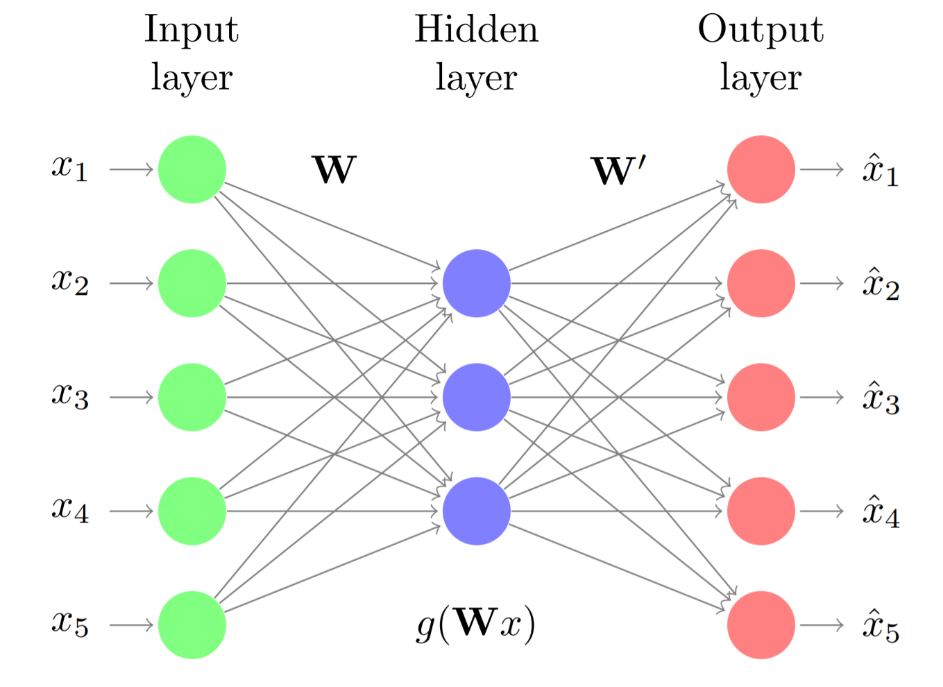
To ensure that the reconstructed output is as similar as possible to the input, the model must learn to capture as much information as possible in the intermediate zone. Once trained, the output of the central layer of the autoencoder (the layer with the fewest neurons) is a representation of the input data but with dimensionality equal to the number of neurons in this layer.
The main advantage of autoencoders is that they have no restriction on the type of relationships they can learn, therefore, unlike PCA, dimensionality reduction can include non-linear relationships. The disadvantage is their high risk of overfitting, so it is recommended to use few epochs and always evaluate the evolution of the error using a validation set.
In the case of using linear activation functions, the variables generated in the bottleneck (the layer with the fewest neurons) are very similar to the principal components of a PCA but without necessarily having to be orthogonal to each other.
Libraries
One of the implementations of autoencoders available in Python is found in the H2O library. This library enables the creation of neural networks with autoencoder architecture, among other machine learning models, and allows for easy extraction of reconstruction errors.
# Installation
# ==============================================================================
#!pip install requests
#!pip install tabulate
#!pip install "colorama>=0.3.8"
#!pip install future
#!pip uninstall h2o
#!pip install -f http://h2o-release.s3.amazonaws.com/h2o/latest_stable_Py.html h2o
# Data processing
# ==============================================================================
import numpy as np
import pandas as pd
from mat4py import loadmat
# Graphics
# ==============================================================================
import matplotlib.pyplot as plt
plt.style.use('fivethirtyeight')
plt.rcParams['lines.linewidth'] = 1.5
plt.rcParams['font.size'] = 8
import seaborn as sns
# Preprocessing and modeling
# ==============================================================================
import h2o
from h2o.estimators.deeplearning import H2OAutoEncoderEstimator
# Warnings configuration
# ==============================================================================
import warnings
warnings.filterwarnings('once')
Data
The data used were obtained from Outlier Detection DataSets (ODDS), a repository with data commonly used to compare the ability of different algorithms to identify anomalies (outliers). Shebuti Rayana (2016). ODDS Library. Stony Brook, NY: Stony Brook University, Department of Computer Science.
All these datasets are labeled, it is known whether the observations are anomalies or not (variable y). Although the methods described in the document are unsupervised, i.e., they do not use the response variable, knowing the true classification allows evaluating their ability to correctly identify anomalies.
- Cardiotocography dataset link:
- Number of observations: 1831
- Number of variables: 21
- Number of outliers: 176 (9.6%)
- y: 1 = outliers, 0 = inliers
- Notes: all variables are centered and scaled (mean 0, sd 1).
- Reference: C. C. Aggarwal and S. Sathe, "Theoretical foundations and algorithms for outlier ensembles." ACM SIGKDD Explorations Newsletter, vol. 17, no. 1, pp. 24–47, 2015. Saket Sathe and Charu C. Aggarwal. LODES: Local Density meets Spectral Outlier Detection. SIAM Conference on Data Mining, 2016.
The data is available in MATLAB format (.mat). To read its content the loadmat() function from the mat4py package is used.
# Data reading
# ==============================================================================
cardio = loadmat(filename='cardio.mat')
X = pd.DataFrame(cardio['X'])
X.columns = ["col_" + str(i) for i in X.columns]
y = pd.Series(np.array(cardio['y']).flatten(), name='y')
# Creating a local H2O cluster
# ==============================================================================
h2o.init(
ip = "localhost",
# Number of threads to use (1 = single core, -1 = all available cores).
nthreads = 1,
# Maximum memory available for the cluster.
max_mem_size = "4g",
verbose = False
)
# Remove data from the cluster in case it had already been started.
# ==============================================================================
h2o.remove_all()
h2o.no_progress()
# Transfer data to h2o cluster
# ==============================================================================
X = h2o.H2OFrame(python_obj= X)
# Splitting observations into training and test sets
# ==============================================================================
X_train, X_test = X.split_frame(
ratios=[0.8],
destination_frames= ["datos_train_H2O", "datos_test_H2O"],
seed = 123
)
Autoencoder model
# Training the autoencoder model
# ==============================================================================
# Hyperparameters:
# - hidden=[10, 3, 10]: symmetric architecture with bottleneck of 3 dimensions
# - l1 and l2: regularization to prevent overfitting
# - activation="Tanh": allows capturing non-linear relationships
autoencoder = H2OAutoEncoderEstimator(
activation = "Tanh",
standardize = True,
l1 = 0.01,
l2 = 0.01,
hidden = [10, 3, 10],
epochs = 100,
ignore_const_cols = False,
score_each_iteration = True,
seed = 12345
)
autoencoder.train(
x = X.columns,
training_frame = X_train,
validation_frame = X_test,
max_runtime_secs = None,
ignored_columns = None,
verbose = False
)
autoencoder.summary()
| layer | units | type | dropout | l1 | l2 | mean_rate | rate_rms | momentum | mean_weight | weight_rms | mean_bias | bias_rms | |
|---|---|---|---|---|---|---|---|---|---|---|---|---|---|
| 1 | 21 | Input | 0.0 | ||||||||||
| 2 | 10 | Tanh | 0.0 | 0.01 | 0.01 | 0.0596206 | 0.0131358 | 0.0 | -0.0006532 | 0.0538940 | 0.0038406 | 0.0113920 | |
| 3 | 3 | Tanh | 0.0 | 0.01 | 0.01 | 0.0617362 | 0.0088655 | 0.0 | -0.0384981 | 0.2068415 | -0.0096374 | 0.0139275 | |
| 4 | 10 | Tanh | 0.0 | 0.01 | 0.01 | 0.0607378 | 0.0105192 | 0.0 | 0.0415092 | 0.2210941 | -0.0016290 | 0.0054258 | |
| 5 | 21 | Tanh | 0.01 | 0.01 | 0.0562047 | 0.0162091 | 0.0 | 0.0018195 | 0.0738565 | 0.0240189 | 0.0567052 |
Diagnostics
To identify the appropriate number of epochs, the evolution of training and validation error is used.
fig, ax = plt.subplots(1, 1, figsize=(6, 3))
autoencoder.scoring_history().plot(x='epochs', y='training_rmse', ax=ax)
autoencoder.scoring_history().plot(x='epochs', y='validation_rmse', ax=ax)
ax.set_title('Evolution of training and validation error');

After 15 epochs, the reduction in rmse is minimal. Once the optimal number of epochs has been identified, the model is retrained, this time with all the data.
# Training the final model
# ==============================================================================
autoencoder = H2OAutoEncoderEstimator(
activation = "Tanh",
standardize = True,
l1 = 0.01,
l2 = 0.01,
hidden = [10, 3, 10],
epochs = 15,
ignore_const_cols = False,
score_each_iteration = True,
seed = 12345
)
autoencoder.train(
x = X.columns,
training_frame = X,
verbose = False
)
autoencoder
Model Details ============= H2OAutoEncoderEstimator : Deep Learning Model Key: DeepLearning_model_python_1769121800517_2
| layer | units | type | dropout | l1 | l2 | mean_rate | rate_rms | momentum | mean_weight | weight_rms | mean_bias | bias_rms | |
|---|---|---|---|---|---|---|---|---|---|---|---|---|---|
| 1 | 21 | Input | 0.0 | ||||||||||
| 2 | 10 | Tanh | 0.0 | 0.01 | 0.01 | 0.0546123 | 0.0145504 | 0.0 | -0.0027062 | 0.0610989 | 0.0004966 | 0.0013961 | |
| 3 | 3 | Tanh | 0.0 | 0.01 | 0.01 | 0.0555454 | 0.0143439 | 0.0 | -0.0217032 | 0.2094431 | -0.0002308 | 0.0010188 | |
| 4 | 10 | Tanh | 0.0 | 0.01 | 0.01 | 0.0553020 | 0.0141562 | 0.0 | -0.0285638 | 0.2274879 | -0.0002672 | 0.0022489 | |
| 5 | 21 | Tanh | 0.01 | 0.01 | 0.0486640 | 0.0202909 | 0.0 | -0.0017924 | 0.0721088 | 0.0165920 | 0.0506570 |
ModelMetricsAutoEncoder: deeplearning ** Reported on train data. ** MSE: 0.02449035729645243 RMSE: 0.15649395290698115
| timestamp | duration | training_speed | epochs | iterations | samples | training_rmse | training_mse | |
|---|---|---|---|---|---|---|---|---|
| 2026-01-22 23:43:39 | 0.124 sec | 0.00000 obs/sec | 0.0 | 0 | 0.0 | 0.2159487 | 0.0466338 | |
| 2026-01-22 23:43:39 | 0.314 sec | 15715 obs/sec | 1.5106499 | 1 | 2766.0 | 0.1582957 | 0.0250575 | |
| 2026-01-22 23:43:39 | 0.459 sec | 17756 obs/sec | 2.9868924 | 2 | 5469.0 | 0.1582393 | 0.0250397 | |
| 2026-01-22 23:43:40 | 0.620 sec | 17947 obs/sec | 4.4893501 | 3 | 8220.0 | 0.1564940 | 0.0244904 | |
| 2026-01-22 23:43:40 | 0.737 sec | 19328 obs/sec | 5.9748771 | 4 | 10940.0 | 0.1593714 | 0.0253993 | |
| 2026-01-22 23:43:40 | 0.853 sec | 20418 obs/sec | 7.4937193 | 5 | 13721.0 | 0.1592932 | 0.0253743 | |
| 2026-01-22 23:43:40 | 0.971 sec | 21080 obs/sec | 9.0032769 | 6 | 16485.0 | 0.1587339 | 0.0251965 | |
| 2026-01-22 23:43:40 | 1.107 sec | 21271 obs/sec | 10.4789732 | 7 | 19187.0 | 0.1576803 | 0.0248631 | |
| 2026-01-22 23:43:40 | 1.257 sec | 21121 obs/sec | 11.9623157 | 8 | 21903.0 | 0.1573945 | 0.0247730 | |
| 2026-01-22 23:43:40 | 1.413 sec | 20928 obs/sec | 13.4533042 | 9 | 24633.0 | 0.1566658 | 0.0245442 | |
| 2026-01-22 23:43:40 | 1.553 sec | 21026 obs/sec | 14.9404697 | 10 | 27356.0 | 0.1568127 | 0.0245902 | |
| 2026-01-22 23:43:41 | 1.681 sec | 21211 obs/sec | 16.4385582 | 11 | 30099.0 | 0.1576032 | 0.0248388 | |
| 2026-01-22 23:43:41 | 1.695 sec | 21122 obs/sec | 16.4385582 | 11 | 30099.0 | 0.1564940 | 0.0244904 |
| variable | relative_importance | scaled_importance | percentage |
|---|---|---|---|
| col_20 | 1.0 | 1.0 | 0.3892533 |
| col_12 | 0.5891169 | 0.5891169 | 0.2293157 |
| col_11 | 0.2280840 | 0.2280840 | 0.0887824 |
| col_4 | 0.1004292 | 0.1004292 | 0.0390924 |
| col_14 | 0.0901291 | 0.0901291 | 0.0350830 |
| col_8 | 0.0489400 | 0.0489400 | 0.0190501 |
| col_0 | 0.0388093 | 0.0388093 | 0.0151067 |
| col_1 | 0.0364324 | 0.0364324 | 0.0141814 |
| col_6 | 0.0353312 | 0.0353312 | 0.0137528 |
| col_2 | 0.0346268 | 0.0346268 | 0.0134786 |
| --- | --- | --- | --- |
| col_17 | 0.0340820 | 0.0340820 | 0.0132665 |
| col_7 | 0.0339693 | 0.0339693 | 0.0132226 |
| col_5 | 0.0337636 | 0.0337636 | 0.0131426 |
| col_15 | 0.0336859 | 0.0336859 | 0.0131124 |
| col_18 | 0.0334737 | 0.0334737 | 0.0130297 |
| col_13 | 0.0332283 | 0.0332283 | 0.0129342 |
| col_19 | 0.0330312 | 0.0330312 | 0.0128575 |
| col_9 | 0.0329193 | 0.0329193 | 0.0128140 |
| col_10 | 0.0327039 | 0.0327039 | 0.0127301 |
| col_3 | 0.0320731 | 0.0320731 | 0.0124846 |
[21 rows x 4 columns]
[tips] Use `model.explain()` to inspect the model. -- Use `h2o.display.toggle_user_tips()` to switch on/off this section.
Reconstruction error
The anomaly() method of an H2OAutoEncoderEstimator model allows obtaining the reconstruction error. To do this, it automatically performs the encoding, decoding, and comparison of the reconstructed values with the original values.
The mean squared reconstruction error of an observation is calculated as the average of the squared differences between the original value of its variables and the reconstructed value, i.e., the average of the reconstruction errors of all its variables squared.
# Calculating reconstruction error
# ==============================================================================
reconstruction_error = autoencoder.anomaly(test_data = X)
reconstruction_error = reconstruction_error.as_data_frame()
reconstruction_error = reconstruction_error['Reconstruction.MSE']
Anomaly detection
Once the reconstruction error has been calculated, it can be used as a criterion to identify anomalies. Assuming that the dimensionality reduction has been performed so that most of the data (the normal ones) are well represented, those observations with the highest reconstruction error should be the most atypical.
In practice, if this detection strategy is being used, it is because labeled data is not available, i.e., it is not known which observations are actually anomalies. However, since the true classification is available in this example, it can be verified whether the anomalous data actually have higher reconstruction errors.
# Distribution of reconstruction error in anomalies and non-anomalies
# ==============================================================================
results = pd.DataFrame({
'reconstruction_error': reconstruction_error,
'anomaly': y.astype(str)
})
fig, ax = plt.subplots(figsize=(5, 3))
sns.boxplot(
x = 'reconstruction_error',
y = 'anomaly',
hue = 'anomaly',
data = results,
ax = ax
)
ax.set_xscale("log")
ax.set_title('Distribution of reconstruction errors')
ax.set_xlabel('log(Reconstruction error)')
ax.set_ylabel('classification (0 = normal, 1 = anomaly)');

The distribution of reconstruction errors in the anomaly group (1) is clearly higher. However, since there is overlap, if the n observations with the highest reconstruction error are classified as anomalies, false positive errors would be incurred.
According to the documentation, the Cardiotocography dataset contains 176 anomalies. See the resulting confusion matrix if the 176 observations with the highest reconstruction error are classified as anomalies.
# Confusion matrix of final classification
# ==============================================================================
results = (
results
.sort_values('reconstruction_error', ascending=False)
.reset_index(drop=True)
)
results['classification'] = np.where(results.index <= 176, 1, 0)
pd.crosstab(
results['anomaly'],
results['classification'],
rownames=['true value'],
colnames=['prediction']
)
| prediction | 0 | 1 |
|---|---|---|
| true value | ||
| 0.0 | 1608 | 47 |
| 1.0 | 46 | 130 |
Of the 177 observations identified as anomalies, 73% (130/177) are anomalies. The model manages to identify a high percentage of the anomalies, even so, it has difficulty completely separating the anomalies from normal observations.
Iterative retraining
The previous autoencoder model was trained using all observations, including potential anomalies. Since the goal is to generate a projection space for "normal" data, the result can be improved by retraining the model but this time excluding the $n$ observations with the highest reconstruction error (potential anomalies).
Anomaly detection is repeated but this time discarding observations with a reconstruction error above the 0.8 quantile. With this threshold, approximately 20% of the most atypical observations are removed, allowing the model to focus on learning the structure of the normal data.
# Removing observations with reconstruction error above the 0.8 quantile
# ==============================================================================
quantile = np.quantile(a=reconstruction_error, q=0.8)
X_pandas = X.as_data_frame()
X_trimmed = X_pandas.loc[reconstruction_error < quantile, :]
X_trimmed = h2o.H2OFrame(python_obj=X_trimmed)
# Retraining the model with filtered data
# ==============================================================================
# The model is retrained using only observations with lower reconstruction error
autoencoder.train(
x = X_trimmed.columns,
training_frame = X_trimmed,
verbose = False
)
Model Details ============= H2OAutoEncoderEstimator : Deep Learning Model Key: DeepLearning_model_python_1769121800517_3
| layer | units | type | dropout | l1 | l2 | mean_rate | rate_rms | momentum | mean_weight | weight_rms | mean_bias | bias_rms | |
|---|---|---|---|---|---|---|---|---|---|---|---|---|---|
| 1 | 21 | Input | 0.0 | ||||||||||
| 2 | 10 | Tanh | 0.0 | 0.01 | 0.01 | 0.0291871 | 0.0219678 | 0.0 | -0.0055397 | 0.0933082 | -0.0022585 | 0.0170172 | |
| 3 | 3 | Tanh | 0.0 | 0.01 | 0.01 | 0.0169608 | 0.0053685 | 0.0 | -0.0130222 | 0.2824453 | -0.0043661 | 0.0221675 | |
| 4 | 10 | Tanh | 0.0 | 0.01 | 0.01 | 0.0167799 | 0.0084733 | 0.0 | -0.0478559 | 0.2907931 | -0.0030111 | 0.0088228 | |
| 5 | 21 | Tanh | 0.01 | 0.01 | 0.0178878 | 0.0104283 | 0.0 | -0.0072167 | 0.0989479 | 0.0150805 | 0.0496585 |
ModelMetricsAutoEncoder: deeplearning ** Reported on train data. ** MSE: 0.023428990459610305 RMSE: 0.15306531435831666
| timestamp | duration | training_speed | epochs | iterations | samples | training_rmse | training_mse | |
|---|---|---|---|---|---|---|---|---|
| 2026-01-22 23:43:42 | 0.082 sec | 0.00000 obs/sec | 0.0 | 0 | 0.0 | 0.2251519 | 0.0506934 | |
| 2026-01-22 23:43:42 | 0.190 sec | 21777 obs/sec | 1.4726776 | 1 | 2156.0 | 0.1530653 | 0.0234290 | |
| 2026-01-22 23:43:42 | 0.292 sec | 22947 obs/sec | 2.9938525 | 2 | 4383.0 | 0.1596385 | 0.0254845 | |
| 2026-01-22 23:43:43 | 0.403 sec | 22789 obs/sec | 4.5143443 | 3 | 6609.0 | 0.1597282 | 0.0255131 | |
| 2026-01-22 23:43:43 | 0.509 sec | 22766 obs/sec | 6.0027322 | 4 | 8788.0 | 0.1590834 | 0.0253075 | |
| 2026-01-22 23:43:43 | 0.608 sec | 23014 obs/sec | 7.4986339 | 5 | 10978.0 | 0.1581181 | 0.0250013 | |
| 2026-01-22 23:43:43 | 0.705 sec | 23396 obs/sec | 8.9972678 | 6 | 13172.0 | 0.1596812 | 0.0254981 | |
| 2026-01-22 23:43:43 | 0.804 sec | 23548 obs/sec | 10.5034153 | 7 | 15377.0 | 0.1597646 | 0.0255247 | |
| 2026-01-22 23:43:43 | 0.922 sec | 23105 obs/sec | 11.9945355 | 8 | 17560.0 | 0.1597635 | 0.0255244 | |
| 2026-01-22 23:43:43 | 1.038 sec | 22852 obs/sec | 13.5020492 | 9 | 19767.0 | 0.1632883 | 0.0266631 | |
| 2026-01-22 23:43:43 | 1.144 sec | 22890 obs/sec | 15.0259563 | 10 | 21998.0 | 0.1580599 | 0.0249829 | |
| 2026-01-22 23:43:43 | 1.160 sec | 22795 obs/sec | 15.0259563 | 10 | 21998.0 | 0.1530653 | 0.0234290 |
| variable | relative_importance | scaled_importance | percentage |
|---|---|---|---|
| col_12 | 1.0 | 1.0 | 0.1526174 |
| col_20 | 0.9821752 | 0.9821752 | 0.1498970 |
| col_0 | 0.7182886 | 0.7182886 | 0.1096233 |
| col_11 | 0.6908948 | 0.6908948 | 0.1054426 |
| col_18 | 0.6157004 | 0.6157004 | 0.0939666 |
| col_4 | 0.5618078 | 0.5618078 | 0.0857417 |
| col_14 | 0.3628029 | 0.3628029 | 0.0553700 |
| col_7 | 0.2872897 | 0.2872897 | 0.0438454 |
| col_16 | 0.2419246 | 0.2419246 | 0.0369219 |
| col_3 | 0.2130911 | 0.2130911 | 0.0325214 |
| --- | --- | --- | --- |
| col_9 | 0.1780681 | 0.1780681 | 0.0271763 |
| col_17 | 0.1570718 | 0.1570718 | 0.0239719 |
| col_19 | 0.1522639 | 0.1522639 | 0.0232381 |
| col_8 | 0.0910602 | 0.0910602 | 0.0138974 |
| col_13 | 0.0448850 | 0.0448850 | 0.0068502 |
| col_10 | 0.0342585 | 0.0342585 | 0.0052284 |
| col_5 | 0.0049315 | 0.0049315 | 0.0007526 |
| col_15 | 0.0036547 | 0.0036547 | 0.0005578 |
| col_2 | 0.0031253 | 0.0031253 | 0.0004770 |
| col_6 | 0.0013269 | 0.0013269 | 0.0002025 |
[21 rows x 4 columns]
[tips] Use `model.explain()` to inspect the model. -- Use `h2o.display.toggle_user_tips()` to switch on/off this section.
# Reconstruction error
# ==============================================================================
reconstruction_error = autoencoder.anomaly(test_data = X)
reconstruction_error = reconstruction_error.as_data_frame()
reconstruction_error = reconstruction_error['Reconstruction.MSE']
# Confusion matrix of classification after retraining
# ==============================================================================
results = pd.DataFrame({
'reconstruction_error' : reconstruction_error,
'anomaly' : y.astype(str)
})
results = (
results
.sort_values('reconstruction_error', ascending=False)
.reset_index(drop=True)
)
results['classification'] = np.where(results.index <= 176, 1, 0)
pd.crosstab(
results['anomaly'],
results['classification'],
rownames=['true value'],
colnames=['prediction']
)
| prediction | 0 | 1 |
|---|---|---|
| true value | ||
| 0.0 | 1617 | 38 |
| 1.0 | 37 | 139 |
After discarding 20% of the observations with the highest error and retraining the autoencoder, an improvement is observed in the model's ability to identify anomalies. Iterative retraining allows the model to specialize in learning the structure of normal data, thus increasing the separation between reconstruction errors of normal and anomalous observations.
✏️ Note
In real scenarios without labels, the number of anomalies to identify must be determined through methods such as error distribution analysis, domain tests, or specific percentiles based on business knowledge.
PyOD
The PyOD library is a Python library specialized in anomaly detection. It provides a wide range of algorithms, both classical and based on deep learning, including autoencoders.
Below is an example of how to use PyOD to detect anomalies with autoencoders on the Cardiotocography dataset.
Libraries
# Libraries
# ==============================================================================
from pyod.models.auto_encoder import AutoEncoder
Data
# Data reading
# ==============================================================================
cardio = loadmat(filename='cardio.mat')
X = pd.DataFrame(cardio['X'])
X.columns = ["col_" + str(i) for i in X.columns]
y = pd.Series(np.array(cardio['y']).flatten(), name='y')
Autoencoder model
# Autoencoder with PyOD
# ==============================================================================
autoencoder_pyod = AutoEncoder(
hidden_neuron_list = [10, 3, 10],
epoch_num = 50,
contamination = 0.1,
preprocessing = True,
hidden_activation_name = 'relu',
batch_norm = True,
dropout_rate = 0.2,
lr = 0.005,
batch_size = 32,
optimizer_name = 'adam',
random_state = 12345
)
autoencoder_pyod.fit(X=X)
Anomaly detection
PyOD models have two prediction methods that return different information. With the predict() method, a binary classification of anomaly (1) or normal (0) is directly returned according to the contamination proportion that was indicated in the model definition.
With the decision_function() method, an anomaly score is obtained for each observation, where higher values indicate a higher probability of being an anomaly. This score can be used to establish custom thresholds or to compare the relative "anomalousness" between observations.
# Anomaly detection: anomaly scores
# ==============================================================================
anomaly_score = autoencoder_pyod.decision_function(X=X)
anomaly_score
array([2.9682167, 3.2247372, 4.0680285, ..., 4.420389 , 4.218177 ,
6.6297894], shape=(1831,), dtype=float32)
# Anomaly detection: binary classification
# ==============================================================================
anomaly_classification = autoencoder_pyod.predict(X=X)
anomaly_classification
array([0, 0, 0, ..., 0, 0, 1], shape=(1831,))
# Confusion matrix of final classification
# ==============================================================================
df_results = pd.DataFrame({
'score' : anomaly_score,
'anomaly' : y.astype(str)
})
df_results = (
df_results
.sort_values('score', ascending=False)
.reset_index(drop=True)
)
df_results['classification'] = np.where(df_results.index <= 176, 1, 0)
pd.crosstab(
df_results['anomaly'],
df_results['classification'],
rownames=['true value'],
colnames=['prediction']
)
| prediction | 0 | 1 |
|---|---|---|
| true value | ||
| 0.0 | 1556 | 99 |
| 1.0 | 98 | 78 |
On this dataset, PyOD's autoencoder achieves worse results than H2O's.
Session information
import session_info
session_info.show(html=False)
----- h2o 3.46.0.9 mat4py 0.6.0 matplotlib 3.10.8 numpy 2.2.6 pandas 2.3.3 pyod 2.0.6 seaborn 0.13.2 session_info v1.0.1 ----- IPython 9.8.0 jupyter_client 8.7.0 jupyter_core 5.9.1 ----- Python 3.13.11 | packaged by Anaconda, Inc. | (main, Dec 10 2025, 21:28:48) [GCC 14.3.0] Linux-6.14.0-37-generic-x86_64-with-glibc2.39 ----- Session information updated at 2026-01-22 23:44
Bibliography
Outlier Analysis Aggarwal, Charu C.
Outlier Ensembles: An Introduction by Charu C. Aggarwal, Saket Sathe
Introduction to Machine Learning with Python: A Guide for Data Scientists
Python Data Science Handbook by Jake VanderPlas
Citation instructions
How to cite this document?
If you use this document or any part of it, we would appreciate if you cite it. Thank you very much!
Anomaly detection with autoencoders and Python by Joaquín Amat Rodrigo, available under an Attribution-NonCommercial-ShareAlike 4.0 International (CC BY-NC-SA 4.0 DEED) license at https://www.cienciadedatos.net/documentos/py32-deteccion-anomalias-autoencoder-python.html
Did you like the article? Your help is important
Your contribution will help me continue generating free informative content. Thank you very much! 😊


This document created by Joaquín Amat Rodrigo is licensed under Attribution-NonCommercial-ShareAlike 4.0 International.
You are free to:
-
Share: copy and redistribute the material in any medium or format.
-
Adapt: remix, transform, and build upon the material.
Under the following terms:
-
Attribution: You must give appropriate credit, provide a link to the license, and indicate if changes were made. You may do so in any reasonable manner, but not in any way that suggests the licensor endorses you or your use.
-
NonCommercial: You may not use the material for commercial purposes.
-
ShareAlike: If you remix, transform, or build upon the material, you must distribute your contributions under the same license as the original.