More about machine learning: Machine Learning with Python
- Linear regression
- Logistic regression
- Decision trees
- Random forest
- Gradient boosting
- Machine learning with Python and Scikitlearn
- Neural Networks
- Principal Component Analysis (PCA)
- Clustering with python
- Anomaly detection with PCA
- Face Detection and Recognition
- Introduction to Graphs and Networks
Introduction
Support Vector Machines (SVMs) is a classification and regression algorithm developed in the 1990s in the field of computer science. Although initially developed as a binary classification method, its application has been extended to multi-class classification problems and regression. SVMs have proven to be one of the best classifiers for a wide range of situations, making them one of the reference methods in statistical learning and machine learning.
Support Vector Machines are based on the Maximal Margin Classifier, which in turn is based on the concept of a hyperplane. Throughout this document, each of these concepts is introduced in order. Understanding the fundamentals of SVMs requires solid knowledge in linear algebra and optimization. This document does not delve into the mathematical aspects, but a detailed description can be found in the book Support Vector Machines Succinctly by Alexandre Kowalczyk.
The Scikit Learn library contains Python implementations of the main SVM algorithms.
Hyperplane and Maximal Margin Classifier
In a p-dimensional space, a hyperplane is defined as a flat and affine subspace of dimension $p-1$. The term affine means that the subspace does not necessarily pass through the origin. In a two-dimensional space, the hyperplane is a one-dimensional subspace, i.e., a line. In a three-dimensional space, a hyperplane is a two-dimensional subspace, a conventional plane. For dimensions $p>3$ it is not intuitive to visualize a hyperplane, but the concept of a $p-1$ dimensional subspace remains.
The mathematical definition of a hyperplane is quite simple. In the case of two dimensions, the hyperplane is described according to the equation of a line:
$$\beta_0 + \beta_1x_1 + \beta_2x_2 = 0$$Given the parameters $\beta_0$, $\beta_1$, and $\beta_2$, all pairs of values $\textbf{x} = (x_1, x_2)$ that satisfy the equality are points on the hyperplane. This equation can be generalized to p-dimensions:
$$\beta_0 + \beta_1x_1 + \beta_2x_2 + ... + \beta_px_p = 0$$and similarly, all points defined by the vector $\textbf{x} = (x_1, x_2,...,x_p)$ that satisfy the equation belong to the hyperplane.
When $\textbf{x}$ does not satisfy the equation:
$$\beta_0 + \beta_1x_1 + \beta_2x_2 + ... + \beta_px_p < 0$$or
$$\beta_0 + \beta_1x_1 + \beta_2x_2 + ... + \beta_px_p > 0$$the point $\textbf{x}$ falls on one side or the other of the hyperplane. Thus, a hyperplane can be understood to divide a p-dimensional space into two halves. To determine on which side of the hyperplane a given point $\textbf{x}$ is located, one simply needs to calculate the sign of the equation.
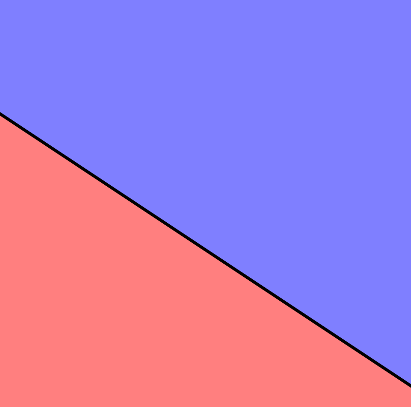
The following image shows the hyperplane of a two-dimensional space. The equation describing the hyperplane (a line) is $1 + 2x_1 + 3x_2 = 0$. The blue region represents the space where all points satisfy $1 + 2x_1 + 3x_2 > 0$, and the red region represents the space for points where $1 + 2x_1 + 3x_2 < 0$.
Binary Classification Using a Hyperplane
When there are $n$ observations, each with $p$ predictors and whose response variable has two levels (hereinafter identified as $+1$ and $-1$), hyperplanes can be used to construct a classifier that allows predicting which group an observation belongs to based on its predictors.
To facilitate understanding, the following explanations are based on a two-dimensional space, where a hyperplane is a line. However, the same concepts apply to higher dimensions.
PERFECTLY LINEARLY SEPARABLE CASES
If the distribution of the observations is such that they can be perfectly separated linearly into the two classes ($+1$ and $-1$), then a separating hyperplane satisfies:
$$\beta_0 + \beta_1x_1 + \beta_2x_2 + ... + \beta_px_p > 0, \ if \ y_i=1$$$$\beta_0 + \beta_1x_1 + \beta_2x_2 + ... + \beta_px_p < 0, \ if \ y_i=-1$$Under this scenario, the simplest classifier consists of assigning each observation to a class depending on the side of the hyperplane where it is located. That is, the observation $\textbf{x}^*$ is classified according to the sign of the function $f(\textbf{x}^*) = \beta_0 + \beta_1x^*_1 + \beta_2x^*_2 + ... + \beta_px^*_p$. If $f(\textbf{x}^*)$ is positive, the observation is assigned to class $+1$; if negative, to class $-1$. Furthermore, the magnitude of $f(\textbf{x}^*)$ indicates how far the observation is from the hyperplane and thus the confidence of the classification (not to be confused with a probability value).
The definition of a hyperplane for perfectly linearly separable cases results in an infinite number of possible hyperplanes, making it necessary to have a method that allows selecting one of them as the optimal classifier.
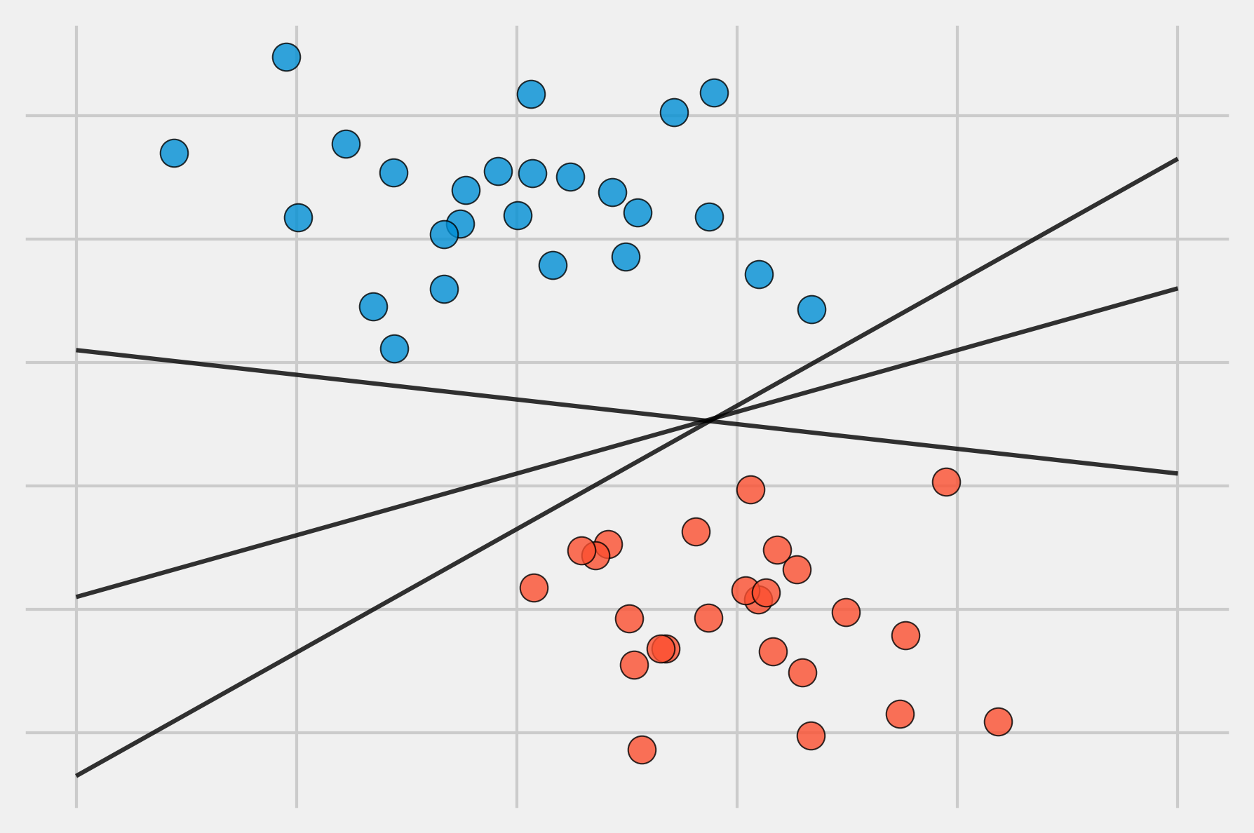
The solution to this problem consists of selecting as the optimal classifier the hyperplane that is furthest away from all training observations. This is known as the maximal margin hyperplane or optimal separating hyperplane. To identify it, the perpendicular distance from each observation to a given hyperplane must be calculated. The smallest of these distances (known as the margin) determines how far the hyperplane is from the training observations. Thus, the maximal margin hyperplane is defined as the hyperplane that achieves the largest margin, meaning the minimum distance between the hyperplane and the observations is as large as possible. Although this idea sounds reasonable, it cannot be applied as stated because there would be infinite hyperplanes against which to measure distances. Instead, dual optimization methods are used.
The image above shows the maximal margin hyperplane, formed by the hyperplane (solid black line) and its margin (the two dashed lines). The three observations equidistant from the maximal margin hyperplane that lie along the dashed lines are known as support vectors, as they are vectors in a p-dimensional space and support (define) the maximal margin hyperplane. Any modification to these observations (support vectors) leads to changes in the maximal margin hyperplane. However, modifications to observations that are not support vectors have no impact on the hyperplane.
QUASI-LINEARLY SEPARABLE CASES
The maximal margin hyperplane described in the previous section is a very simple and natural form of classification as long as there exists a separating hyperplane. In the vast majority of real cases, the data cannot be perfectly separated linearly, so there is no separating hyperplane and a maximal margin hyperplane cannot be obtained.
To solve these situations, the concept of maximal margin hyperplane can be extended to obtain a hyperplane that "almost" separates the classes, but allowing a few errors to be made. This type of hyperplane is known as a Support Vector Classifier or Soft Margin.
Support Vector Classifier or Soft Margin SVM
The Maximal Margin Classifier described in the previous section has little practical application, as cases where classes are perfectly and linearly separable are rare. In fact, even when these ideal conditions are met, where there exists a hyperplane capable of perfectly separating the observations into two classes, this approach still has two drawbacks:
Since the hyperplane must perfectly separate the observations, it is very sensitive to variations in the data. Including a new observation can lead to very large changes in the separating hyperplane (poor robustness).
Having the maximal margin hyperplane fit perfectly to the training observations to separate them all correctly usually leads to overfitting problems.
For these reasons, it is preferable to create a classifier based on a hyperplane that, although not perfectly separating the two classes, is more robust and has greater predictive capacity when applied to new observations (fewer overfitting problems). This is exactly what support vector classifiers achieve, also known as soft margin classifiers or Support Vector Classifiers. To achieve this, instead of seeking the widest classification margin that ensures observations are on the correct side of the margin, certain observations are allowed to be on the incorrect side of the margin or even of the hyperplane.
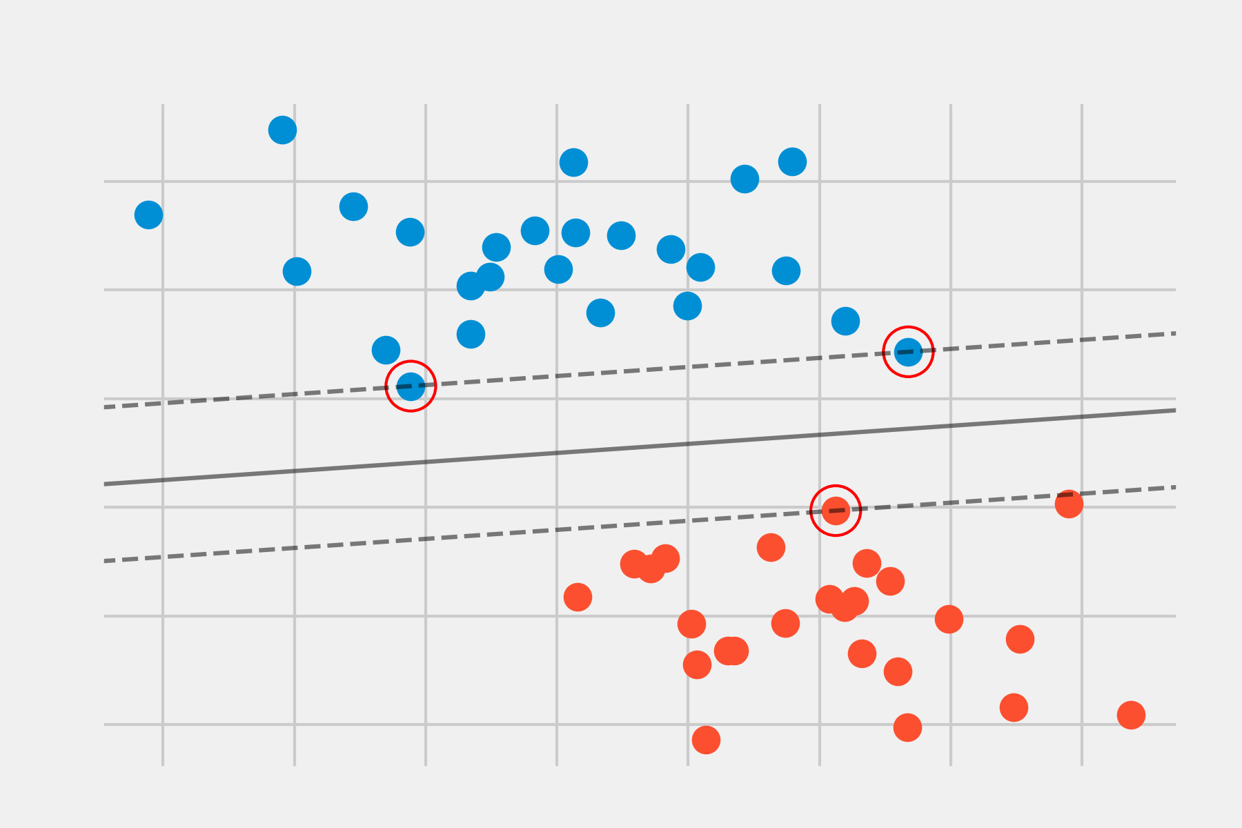
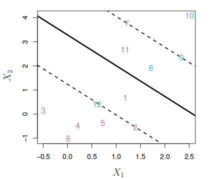
The following image shows a support vector classifier fitted to a small set of observations. The solid line represents the hyperplane and the dashed lines represent the margin on each side. Observations 2, 3, 4, 5, 6, 7, 9, and 10 are on the correct side of the margin (also of the hyperplane), so they are correctly classified. Observations 1 and 8, although within the margin, are on the correct side of the hyperplane, so they are also correctly classified. Observations 11 and 12 are on the wrong side of the hyperplane, so their classification is incorrect. All those observations that, whether inside or outside the margin, are on the incorrect side of the hyperplane correspond to misclassified training observations.
The identification of the hyperplane that correctly classifies most observations except for a few is a convex optimization problem. While the mathematical demonstration is beyond the scope of this introduction, it is important to mention that the process includes a hyperparameter called $C$. $C$ controls the number and severity of margin (and hyperplane) violations that are tolerated in the fitting process. If $C= \infty$, no margin violations are allowed, and therefore the result is equivalent to the Maximal Margin Classifier (noting that this solution is only possible if the classes are perfectly separable). The closer $C$ approaches zero, the less errors are penalized, and more observations can be on the incorrect side of the margin or even the hyperplane. $C$ is ultimately the hyperparameter responsible for controlling the balance between bias and variance of the model. In practice, its optimal value is identified through cross-validation.
The optimization process has the peculiarity that only observations that lie exactly on the margin or that violate it influence the hyperplane. These observations are known as support vectors and are the ones that define the obtained classifier. This is why parameter $C$ controls the balance between bias and variance. When the value of $C$ is small, the margin is wider, and more observations violate the margin, becoming support vectors. The hyperplane is therefore supported by more observations, which increases bias but reduces variance. The larger the value of $C$, the narrower the margin, fewer observations are support vectors, and the resulting classifier has lower bias but higher variance.
Another important property that derives from the hyperplane depending only on a small proportion of observations (support vectors) is its robustness against observations very far from the hyperplane. This makes the support vector classification method different from other methods such as Linear Discriminant Analysis (LDA), where the classification rule depends on the mean of all observations.
Note: in the book Introduction to Statistical Learning, a term $C$ is used that is equivalent to the inverse of the one described in this document.
Support Vector Machines
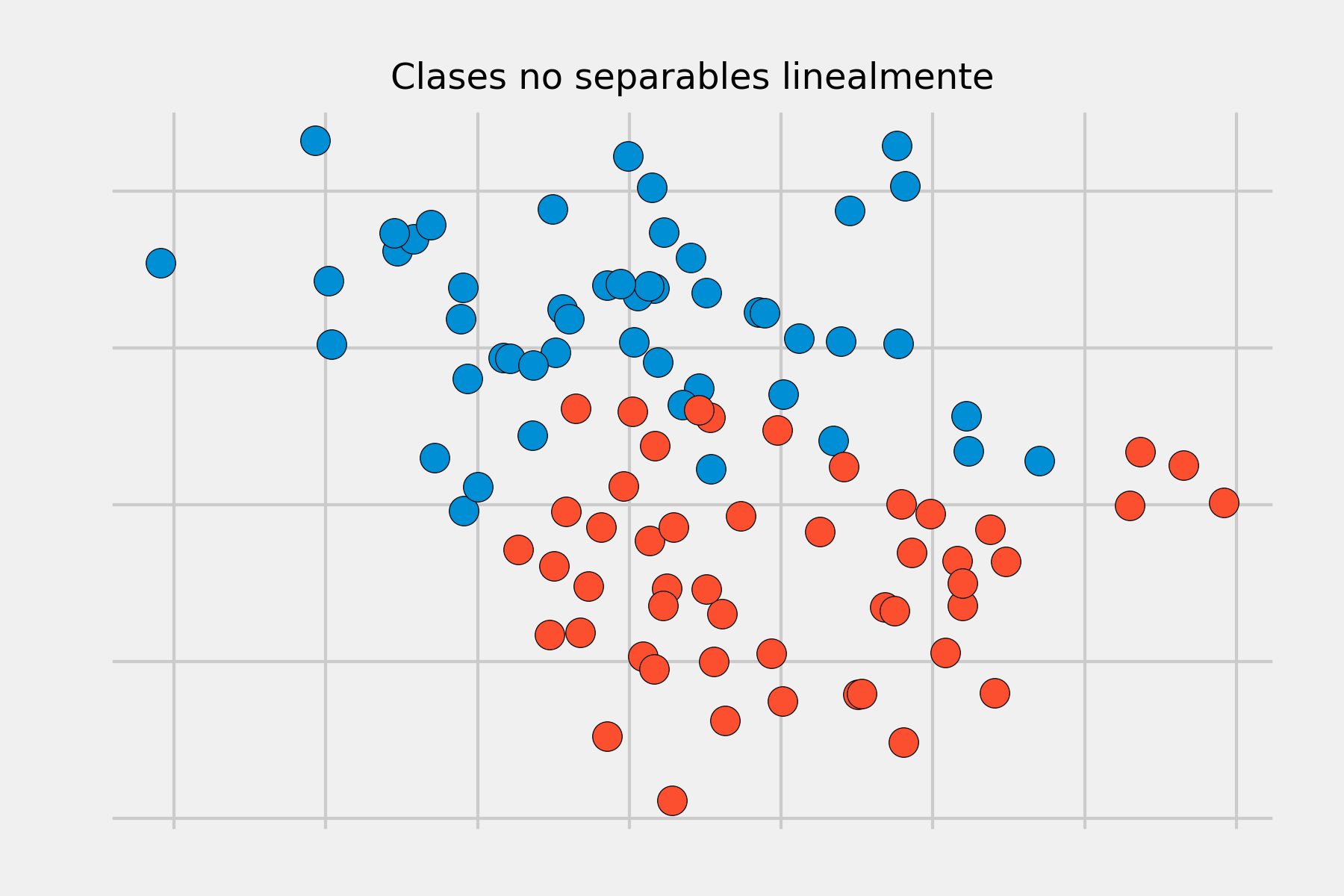
The Support Vector Classifier described in the previous sections achieves good results when the boundary separating classes is approximately linear. If it is not, its performance drops drastically. A strategy to deal with scenarios where the separation between groups is of a non-linear type consists of expanding the dimensions of the original space.
The fact that groups are not linearly separable in the original space does not mean they are not separable in a higher-dimensional space. The following images show two groups whose separation in two dimensions is non-linear, but is linear when adding a third dimension.
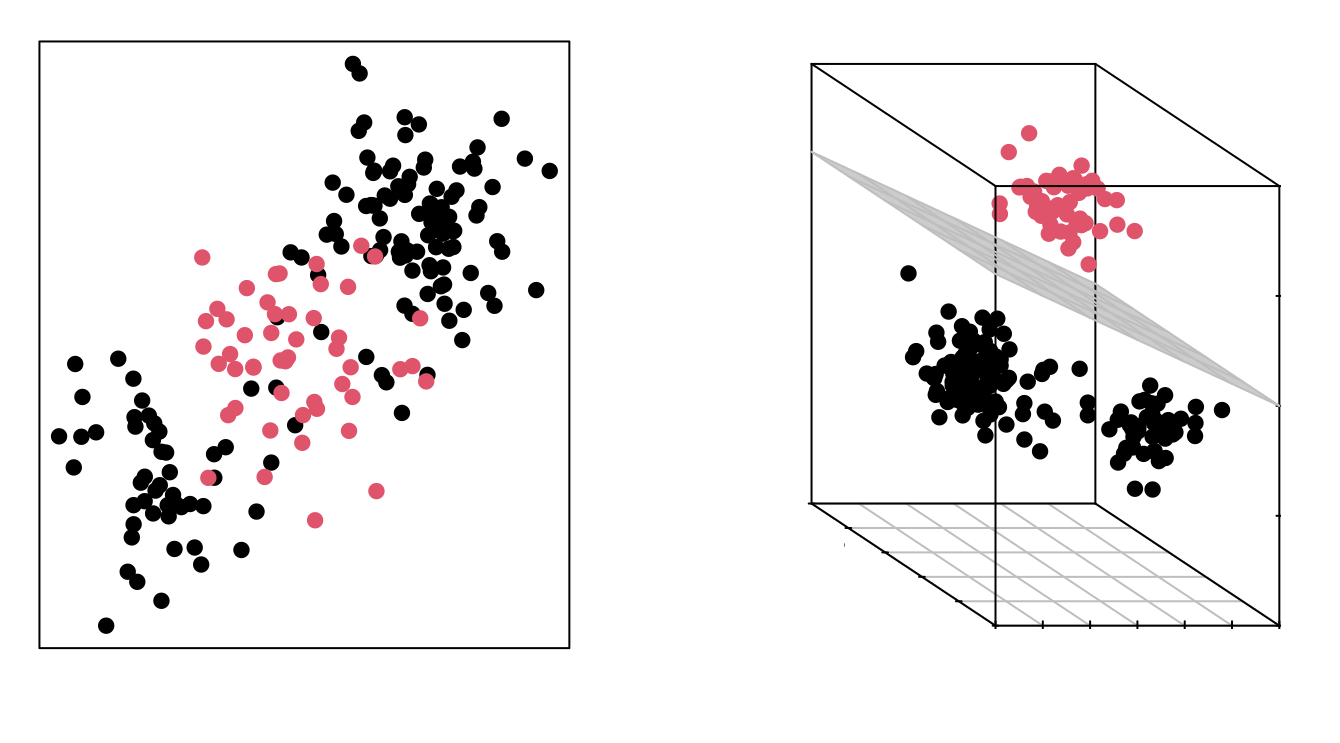
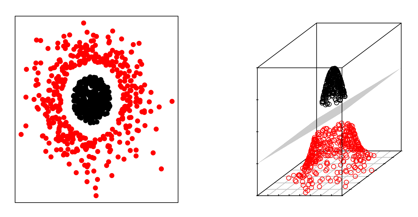
The Support Vector Machines (SVM) method can be considered as an extension of the Support Vector Classifier obtained by increasing the dimension of the data. The linear separation boundaries generated in the expanded space become non-linear separation boundaries when projected into the original space.
Dimensionality Expansion: Kernels
Once it is defined that Support Vector Machines follow the same strategy as the Support Vector Classifier, but by increasing the dimension of the data before applying the algorithm, the immediate question is: How is the dimension increased and what dimension is correct?
The dimension of a dataset can be transformed by combining or modifying any of its dimensions. For example, a two-dimensional space can be transformed into a three-dimensional one by applying the following function:
$$f(x_1,x_2) = (x_1^2, \sqrt{2}x_1x_2, x_2^2) $$This is just one of infinitely many possible transformations. How do we know which one is appropriate? This is where the concept of kernel comes into play. A kernel (K) is a function that returns the result of the dot product between two vectors performed in a new dimensional space different from the original space where the vectors are located. Although we have not gone into detail with the mathematical formulas used to solve the optimization problem, it contains a dot product. If this dot product is replaced by a kernel, the support vectors (and the hyperplane) are obtained directly in the dimension corresponding to the kernel. This is often known as the kernel trick because, with just a slight modification of the original problem, the result can be obtained for any dimension. There are many different kernels, some of the most commonly used are:
Linear kernel
$$K(\textbf{x}, \textbf{x'}) = \textbf{x} \cdot \textbf{x'}$$If a linear kernel is used, the Support Vector Machine classifier obtained is equivalent to the Support Vector Classifier.
Polynomial kernel
$$K(\textbf{x}, \textbf{x'}) = (\textbf{x} \cdot \textbf{x'} + c) ^ d$$When $d = 1$ and $c=0$ are used, the result is the same as that of a linear kernel. If $d>1$, non-linear decision boundaries are generated, increasing the non-linearity as $d$ increases. It is not usually recommended to use values of $d$ greater than 5 due to overfitting problems.
Gaussian Kernel (RBF)
$$K(\textbf{x}, \textbf{x'}) = exp(- \gamma ||\textbf{x} - \textbf{x'}||^2)$$The value of $\gamma$ controls the behavior of the kernel. When it is very small, the final model is equivalent to that obtained with a linear kernel; as its value increases, so does the flexibility of the model.
The described kernels are just a few of the many that exist. Each has a series of hyperparameters whose optimal value can be found through cross-validation. It cannot be said that there is one kernel that surpasses the rest; it depends largely on the nature of the problem being addressed. However, as indicated by the authors of A Practical Guide to Support Vector Classification, it is highly recommended to try the RBF kernel. This kernel has two advantages: it only has two hyperparameters to optimize ($\gamma$ and the penalty $C$ common to all SVMs), and its flexibility can range from a linear classifier to a very complex one.
Multi-class Classification
The concept of a separating hyperplane on which SVMs are based does not naturally generalize to more than two classes. Numerous strategies have been developed to apply this algorithm to multi-class problems, among which the most commonly used are: one-versus-one, one-versus-all, and DAGSVM.
One-versus-one
Suppose a scenario where there are K > 2 classes and the SVM-based classification method is to be applied. The one-versus-one strategy consists of generating a total of K(K-1)/2 SVMs, comparing all possible pairs of classes. To generate a prediction, each of the K(K-1)/2 classifiers is used, recording the number of times the observation is assigned to each class. Finally, the observation is considered to belong to the class to which it has been assigned most frequently. The main disadvantage of this strategy is that the number of models required increases rapidly as the number of classes increases, so it is not applicable in all scenarios.
One-versus-all
This strategy consists of fitting K different SVMs, each comparing one of the K classes against the remaining K-1 classes. As a result, a classification hyperplane is obtained for each class. To obtain a prediction, each of the K classifiers is used, and the observation is assigned to the class for which the prediction is positive. This approach, although simple, can cause inconsistencies, as it may occur that more than one classifier results in a positive prediction, thus assigning the same observation to different classes. Another additional drawback is that each classifier is trained in an imbalanced manner. For example, if the dataset contains 100 classes with 10 observations per class, each classifier is fitted with 10 positive observations and 990 negative observations.
DAGSVM
DAGSVM (Directed Acyclic Graph SVM) is an improvement of the one-versus-one method. The strategy followed is the same, but they manage to reduce its execution time by eliminating unnecessary comparisons through the use of a directed acyclic graph (DAG). Suppose a dataset with four classes (A, B, C, D) and 6 classifiers trained with each possible pair of classes (A-B, A-C, A-D, B-C, B-D, C-D). Comparisons begin with the classifier (A-D) and the result is that the observation belongs to class A, or equivalently, that it does not belong to class D. With this information, all comparisons containing class D can be excluded, since it is known that it does not belong to this group. In the next comparison, the classifier (A-C) is used and it predicts that it is A. With this new information, all comparisons containing C are excluded. Finally, only the classifier (A-B) needs to be used and the observation assigned to the returned result. Following this strategy, instead of using all 6 classifiers, only 3 were necessary. DAGSVM has the same advantages as the one-versus-one method but greatly improving performance.
Computational Cost
Due to the use of kernels, an n x n matrix is involved in fitting an SVM, where n is the number of training observations. For this reason, what most influences the computation time required to train an SVM is the number of observations, not the number of predictors.
Example
For the following example, a dataset published in the book Elements of Statistical Learning is used, which contains simulated observations with a non-linear function in a two-dimensional space (2 predictors). The goal is to train an SVM model capable of classifying the observations.
Libraries
The libraries used in this example are:
# Data manipulation
# ==============================================================================
import pandas as pd
import numpy as np
# Plots
# ==============================================================================
import matplotlib.pyplot as plt
from matplotlib.colors import ListedColormap
from matplotlib.patches import Patch
plt.style.use('fivethirtyeight')
plt.rcParams['lines.linewidth'] = 1.5
plt.rcParams['font.size'] = 8
# Preprocessing and modeling
# ==============================================================================
from sklearn.svm import SVC
from sklearn.model_selection import train_test_split
from sklearn.model_selection import GridSearchCV
from sklearn.metrics import accuracy_score
from sklearn.inspection import DecisionBoundaryDisplay
# Warnings configuration
# ==============================================================================
import warnings
warnings.filterwarnings('once')
Data
# Data
# ==============================================================================
url = (
'https://raw.githubusercontent.com/JoaquinAmatRodrigo/'
'Estadistica-machine-learning-python/master/data/ESL.mixture.csv'
)
data = pd.read_csv(url)
data.head(3)
| X1 | X2 | y | |
|---|---|---|---|
| 0 | 2.526093 | 0.321050 | 0 |
| 1 | 0.366954 | 0.031462 | 0 |
| 2 | 0.768219 | 0.717486 | 0 |
fig, ax = plt.subplots(figsize=(6, 4))
# Get the first two colors from the fivethirtyeight style
fivethirtyeight_colors = plt.rcParams['axes.prop_cycle'].by_key()['color']
custom_cmap = ListedColormap(fivethirtyeight_colors[:2])
ax.scatter(
x = data['X1'],
y = data['X2'],
c = data['y'],
s = 90,
cmap = custom_cmap,
alpha = 0.8,
edgecolors = 'black',
)
legend_elements = [
Patch(facecolor=fivethirtyeight_colors[0], edgecolor='black', label='Class 0'),
Patch(facecolor=fivethirtyeight_colors[1], edgecolor='black', label='Class 1')
]
ax.legend(handles=legend_elements, title='Class', loc='best')
ax.set_title("ESL.mixture Data");

Linear SVM
In Scikit Learn, three different implementations of the Support Vector Machine algorithm can be found:
The
sklearn.svm.SVCandsklearn.svm.NuSVCclasses allow creating SVM classification models using linear, polynomial, radial, or sigmoid kernels. The difference is thatSVCcontrols regularization through theChyperparameter, whileNuSVCdoes so with the maximum number of support vectors allowed.The
sklearn.svm.LinearSVCclass allows fitting SVM models with a linear kernel. It is similar toSVCwhen thekernel='linear'parameter is used, but uses a faster algorithm.
The same implementations are available for regression in the classes: sklearn.svm.SVR, sklearn.svm.NuSVR, and sklearn.svm.LinearSVR.
First, an SVM model with a linear kernel is fitted, and then one with a radial kernel, and the ability of each to correctly classify the observations is compared.
# Split data into train and test
# ==============================================================================
X = data.drop(columns = 'y')
y = data['y']
X_train, X_test, y_train, y_test = train_test_split(
X,
y,
train_size = 0.8,
random_state = 1234,
shuffle = True
)
# Create linear SVM model
# ==============================================================================
model = SVC(C=100, kernel='linear', random_state=123)
model.fit(X_train, y_train)
SVC(C=100, kernel='linear', random_state=123)In a Jupyter environment, please rerun this cell to show the HTML representation or trust the notebook.
On GitHub, the HTML representation is unable to render, please try loading this page with nbviewer.org.
Parameters
| C | 100 | |
| kernel | 'linear' | |
| degree | 3 | |
| gamma | 'scale' | |
| coef0 | 0.0 | |
| shrinking | True | |
| probability | False | |
| tol | 0.001 | |
| cache_size | 200 | |
| class_weight | None | |
| verbose | False | |
| max_iter | -1 | |
| decision_function_shape | 'ovr' | |
| break_ties | False | |
| random_state | 123 |
Since this is a two-dimensional problem, the classification regions can be visualized.
# Graphical representation of classification boundaries
# ==============================================================================
# Grid of values
x = np.linspace(np.min(X_train.X1), np.max(X_train.X1), 50)
y = np.linspace(np.min(X_train.X2), np.max(X_train.X2), 50)
Y, X = np.meshgrid(y, x)
grid = pd.DataFrame(
np.vstack([X.ravel(), Y.ravel()]).T,
columns=['X1', 'X2']
)
# Prediction on grid values
pred_grid = model.predict(grid)
fig, ax = plt.subplots(figsize=(6, 4))
ax.scatter(grid['X1'], grid['X2'], c=pred_grid, cmap=custom_cmap, alpha=0.2)
ax.scatter(X_train['X1'], X_train['X2'], c=y_train, cmap=custom_cmap, alpha=1)
# Support vectors
ax.scatter(
x = model.support_vectors_[:, 0],
y = model.support_vectors_[:, 1],
s = 200,
linewidth = 1,
facecolors = 'none',
edgecolors = 'black'
)
# Separating hyperplane
ax.contour(
X,
Y,
model.decision_function(grid).reshape(X.shape),
colors = 'k',
levels = [-1, 0, 1],
alpha = 0.5,
linestyles = ['--', '-', '--']
)
ax.set_title("Linear SVM Classification Results");

The percentage of correct predictions (accuracy) that the model achieves when predicting test observations is calculated.
# Test predictions
# ==============================================================================
predictions = model.predict(X_test)
predictions
array([1, 1, 0, 0, 0, 0, 0, 1, 1, 0, 0, 0, 0, 1, 0, 1, 1, 1, 0, 1, 0, 0,
1, 0, 1, 1, 0, 1, 0, 0, 0, 1, 1, 1, 0, 1, 0, 1, 1, 0])
# Test accuracy of the model
# ==============================================================================
accuracy = accuracy_score(
y_true = y_test,
y_pred = predictions,
normalize = True
)
print("")
print(f"Test accuracy is: {100*accuracy}%")
Test accuracy is: 70.0%
Radial SVM
The model fitting is repeated, this time using a radial kernel and using cross-validation to identify the optimal penalty value C.
# Hyperparameter grid
# ==============================================================================
param_grid = {'C': np.logspace(-5, 7, 20)}
# Cross-validation search
# ==============================================================================
grid = GridSearchCV(
estimator = SVC(kernel= "rbf", gamma='scale'),
param_grid = param_grid,
scoring = 'accuracy',
n_jobs = -1,
cv = 3,
verbose = 0,
return_train_score = True
)
# Assign result to _ so it's not printed to screen
_ = grid.fit(X=X_train, y=y_train)
# Grid results
# ==============================================================================
results = pd.DataFrame(grid.cv_results_)
(
results.filter(regex = '(param.*|mean_t|std_t)')
.drop(columns = 'params')
.sort_values('mean_test_score', ascending = False)
.head(5)
)
| param_C | mean_test_score | std_test_score | mean_train_score | std_train_score | |
|---|---|---|---|---|---|
| 8 | 1.128838 | 0.762520 | 0.023223 | 0.790778 | 0.035372 |
| 12 | 379.269019 | 0.750641 | 0.076068 | 0.868777 | 0.007168 |
| 7 | 0.263665 | 0.750175 | 0.030408 | 0.778228 | 0.026049 |
| 9 | 4.832930 | 0.744118 | 0.044428 | 0.815729 | 0.026199 |
| 11 | 88.586679 | 0.738062 | 0.064044 | 0.859431 | 0.019840 |
# Best hyperparameters by cross-validation
# ==============================================================================
print("----------------------------------------")
print("Best hyperparameters found (cv)")
print("----------------------------------------")
print(grid.best_params_, ":", grid.best_score_, grid.scoring)
model = grid.best_estimator_
----------------------------------------
Best hyperparameters found (cv)
----------------------------------------
{'C': np.float64(1.1288378916846884)} : 0.7625203820172374 accuracy
# Graphical representation of classification boundaries
# ==============================================================================
# Grid of values
x = np.linspace(np.min(X_train.X1), np.max(X_train.X1), 50)
y = np.linspace(np.min(X_train.X2), np.max(X_train.X2), 50)
Y, X = np.meshgrid(y, x)
grid = pd.DataFrame(np.vstack([X.ravel(), Y.ravel()]).T, columns=['X1', 'X2'])
# Prediction on grid values
pred_grid = model.predict(grid)
fig, ax = plt.subplots(figsize=(6, 4))
ax.scatter(grid['X1'], grid['X2'], c=pred_grid, alpha=0.2, cmap=custom_cmap)
ax.scatter(X_train['X1'], X_train['X2'], c=y_train, alpha=1, cmap=custom_cmap)
# Support vectors
ax.scatter(
model.support_vectors_[:, 0],
model.support_vectors_[:, 1],
s=200,
linewidth=1,
facecolors='none',
edgecolors='black'
)
# Separating hyperplane
ax.contour(
X,
Y,
model.decision_function(grid).reshape(X.shape),
colors='k',
levels=[0],
alpha=0.5,
linestyles='-'
)
ax.set_title("Radial SVM Classification Results");

# Graphical representation using sklearn DecisionBoundaryDisplay
# ==============================================================================
fig, ax = plt.subplots(figsize=(6, 4))
DecisionBoundaryDisplay.from_estimator(
model,
X_train,
cmap=custom_cmap,
alpha=0.3,
ax=ax,
response_method='predict'
)
# Add training points
ax.scatter(
X_train['X1'],
X_train['X2'],
c=y_train,
cmap=custom_cmap,
edgecolors='black',
s=90
)
ax.set_title("Radial SVM Classification Results");

# Test predictions
# ==============================================================================
predictions = model.predict(X_test)
# Test accuracy of the model
# ==============================================================================
accuracy = accuracy_score(
y_true = y_test,
y_pred = predictions,
normalize = True
)
print("")
print(f"Test accuracy is: {100*accuracy}%")
Test accuracy is: 80.0%
# Confusion matrix of test predictions
# ==============================================================================
confusion_matrix = pd.crosstab(
y_test,
predictions,
rownames=['Actual'],
colnames=['Predicted']
)
confusion_matrix
| Predicted | 0 | 1 |
|---|---|---|
| Actual | ||
| 0 | 14 | 3 |
| 1 | 5 | 18 |
Conclusion
With a radial kernel SVM model, 80% of the test observations are correctly classified. The model could be further improved by optimizing the value of the gamma hyperparameter or using another type of kernel.
Session Information
import session_info
session_info.show(html=False)
----- matplotlib 3.10.8 numpy 2.2.6 pandas 2.3.3 session_info v1.0.1 sklearn 1.7.2 ----- IPython 9.8.0 jupyter_client 8.7.0 jupyter_core 5.9.1 ----- Python 3.13.11 | packaged by Anaconda, Inc. | (main, Dec 10 2025, 21:28:48) [GCC 14.3.0] Linux-6.14.0-37-generic-x86_64-with-glibc2.39 ----- Session information updated at 2026-01-07 23:25
Bibliography
Introduction to Machine Learning with Python: A Guide for Data Scientists
Python Data Science Handbook by Jake VanderPlas
Support Vector Machines Succinctly by Alexandre Kowalczyk book
An Introduction to Statistical Learning: with Applications in R (Springer Texts in Statistics)
Citation Instructions
How to cite this document?
If you use this document or any part of it, we appreciate if you cite it. Thank you very much!
Support Vector Machines (SVM) with Python by Joaquín Amat Rodrigo, available under a Attribution-NonCommercial-ShareAlike 4.0 International (CC BY-NC-SA 4.0 DEED) license at https://www.cienciadedatos.net/documentos/py24-svm-python-en.html
Did you like the article? Your help is important
Your contribution will help me continue generating free educational content. Thank you very much! 😊


This document created by Joaquín Amat Rodrigo is licensed under Attribution-NonCommercial-ShareAlike 4.0 International.
You are free to:
-
Share: copy and redistribute the material in any medium or format.
-
Adapt: remix, transform, and build upon the material.
Under the following terms:
-
Attribution: You must give appropriate credit, provide a link to the license, and indicate if changes were made. You may do so in any reasonable manner, but not in any way that suggests the licensor endorses you or your use.
-
Non-Commercial: You may not use the material for commercial purposes.
-
ShareAlike: If you remix, transform, or build upon the material, you must distribute your contributions under the same license as the original.