More about Data Science and Statistics
- Normality Tests
- Equality of variances
- Linear Correlation
- T-test
- ANOVA
- Permutation tests
- Bootstrapping
- Fitting probability distributions
- Kernel Density Estimation (KDE)
- Kolmogorov-Smirnov Test
- Cramer-Von Mises Test
Introduction
This document presents several strategies to compare distributions and detect whether there are differences between them. In practice, this type of comparison can be useful in cases such as:
Determining whether two variables have the same distribution.
Determining whether the same variable is distributed identically across two groups.
Monitoring models in production: in projects involving the creation and deployment of predictive models, models are trained with historical data assuming that the predictor variables will maintain the same behavior in the near future. How can we detect if this ceases to be true? What if a variable starts behaving differently? Detecting these changes can be used as an alarm to indicate the need to retrain models, either in an automated way or through new studies.
Finding variables with different behavior between two scenarios: in industrial settings, it is common to have multiple production lines that supposedly perform exactly the same process. However, one of the lines often generates different results. One way to discover the reason for this difference is by comparing the variables measured on each line to identify which ones differ to a greater degree.
Multiple strategies exist to address these questions. One of the most commonly used approaches is to compare centrality statistics (mean, median...) or dispersion statistics (standard deviation, interquartile range...). This strategy has the advantage of being easy to implement and interpret. However, each of these statistics only considers one type of difference, so depending on which one is used, important changes may be ignored. For example, two very different distributions can have the same mean.
Another approach consists of using methods that attempt to quantify the "distance" between distributions, for example the Kolmogorov–Smirnov statistic, which is influenced by both differences in location and shape of the distribution.
As with most statistical tests or methods, there is no one that always outperforms the others. Depending on which change in the distribution is most important to detect, one strategy will be better than another.
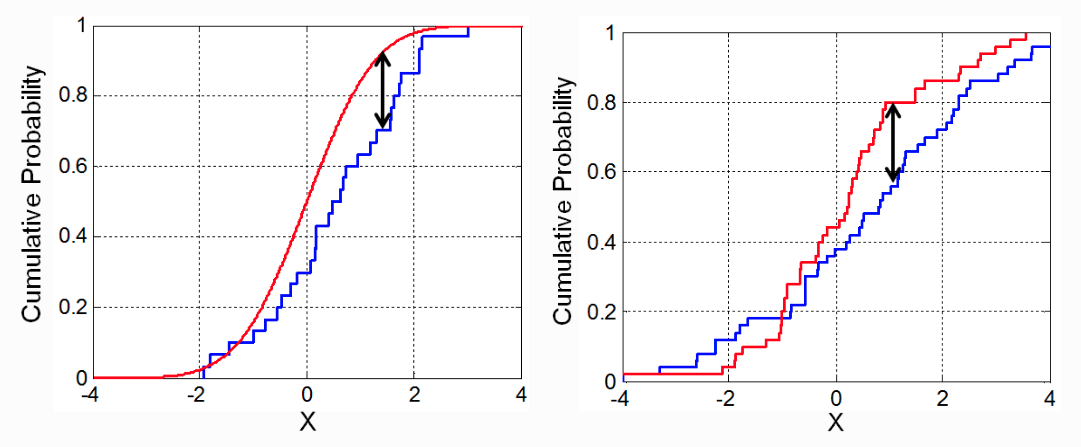
Kolmogorov–Smirnov Distance
The Kolmogorov–Smirnov statistic, also known as Kolmogorov–Smirnov distance (K-S), is defined as the maximum vertical distance between the empirical cumulative distribution functions of two samples, or between an empirical distribution function and a theoretical reference cumulative distribution function. The main advantage of this statistic is that it is sensitive to differences in both the location and shape of the distribution.
Example
A study aims to determine whether the distribution of salaries in Spain has changed between 1989 and 1990. To do this, the Kolmogorov–Smirnov distance is used.
Libraries
The libraries used in this document are:
# Data processing
# ==============================================================================
import numpy as np
import pandas as pd
# Plots
# ==============================================================================
import matplotlib.pyplot as plt
plt.style.use('fivethirtyeight')
plt.rcParams.update({'font.size': 10})
plt.rcParams['lines.linewidth'] = 1
import seaborn as sns
# Modeling and statistical tests
# ==============================================================================
from statsmodels.distributions.empirical_distribution import ECDF
from scipy.stats import ks_2samp
# Warnings configuration
# ==============================================================================
import warnings
warnings.filterwarnings("once")
Data
The Snmesp dataset from the R package plm contains a sample of salaries (on logarithmic scale) paid in Spain during the years 1983 to 1990 (783 observations per year).
# Data
# ==============================================================================
url = ('https://raw.githubusercontent.com/JoaquinAmatRodrigo/'
'Estadistica-machine-learning-python/master/data/Snmesp.csv')
data = pd.read_csv(url)
data['year'] = data['year'].astype(str)
data.info()
<class 'pandas.core.frame.DataFrame'> RangeIndex: 1476 entries, 0 to 1475 Data columns (total 2 columns): # Column Non-Null Count Dtype --- ------ -------------- ----- 0 year 1476 non-null object 1 salary 1476 non-null float64 dtypes: float64(1), object(1) memory usage: 23.2+ KB
Graphical Analysis
# Distribution plots
# ==============================================================================
fig, axs = plt.subplots(nrows=2, ncols=1, figsize=(7, 6))
sns.violinplot(
x = data.salary,
y = data.year,
color = ".8",
ax = axs[0]
)
sns.stripplot(
x = data.salary,
y = data.year,
hue = data.year,
data = data,
size = 4,
jitter = 0.1,
legend = False,
ax = axs[0]
)
axs[0].set_title('Salary distribution by year')
axs[0].set_ylabel('year')
axs[0].set_xlabel('salary')
for year in data.year.unique():
temp_data = data[data.year == year]['salary']
temp_data.plot.kde(ax=axs[1], label=year)
axs[1].plot(temp_data, np.full_like(temp_data, 0), '|k', markeredgewidth=1)
axs[1].set_xlabel('salary')
axs[1].legend()
fig.tight_layout();

Empirical Cumulative Distribution Function
The ECDF() class from the statsmodels library allows fitting the empirical cumulative distribution function from a sample. The result of this function is an ecdf object that behaves similarly to a predictive model, receiving a vector of observations and returning their estimated cumulative probability.
# Fitting ecdf functions with each sample
# ==============================================================================
ecdf_1989 = ECDF(data.loc[data.year == '1989', 'salary'])
ecdf_1990 = ECDF(data.loc[data.year == '1990', 'salary'])
# Estimation of cumulative probability for each observed salary value
# ==============================================================================
salary_grid = np.sort(data.salary.unique())
cumulative_prob_ecdf_1989 = ecdf_1989(salary_grid)
cumulative_prob_ecdf_1990 = ecdf_1990(salary_grid)
# Graphical representation of ecdf curves
# ==============================================================================
fig, ax = plt.subplots(nrows=1, ncols=1, figsize=(6, 4))
ax.plot(salary_grid, cumulative_prob_ecdf_1989, label='1989')
ax.plot(salary_grid, cumulative_prob_ecdf_1990, label='1990')
ax.set_title("Empirical cumulative distribution function of salaries")
ax.set_ylabel("Cumulative probability")
ax.legend();

This same plot can be generated directly with the ecdfplot function from seaborn.
# Graphical representation of ecdf curves
# ==============================================================================
# fig, ax = plt.subplots(nrows=1, ncols=1, figsize=(6, 4))
# sns.ecdfplot(data=data, x="salary", hue='year', ax=ax)
# ax.set_title("Empirical cumulative distribution function of salaries")
# ax.set_ylabel("Cumulative probability");
Calculating the Kolmogorov–Smirnov Distance
To obtain the Kolmogorov–Smirnov distance, first the absolute difference between the cumulative probabilities of each of the ecdf functions is calculated (the absolute difference between each point of the curves) and then the maximum value is identified.
# Kolmogorov–Smirnov distance
# ==============================================================================
abs_diff = np.abs(cumulative_prob_ecdf_1989 - cumulative_prob_ecdf_1990)
ks_distance = np.max(abs_diff)
print(f"Kolmogorov-Smirnov distance: {ks_distance:.4f}")
Kolmogorov-Smirnov distance: 0.1057
Kolmogorov–Smirnov Test
Once the Kolmogorov–Smirnov distance is calculated, it must be determined whether the value of this distance is large enough, considering the available samples, to consider that the two distributions are different. This can be achieved by calculating the probability (p-value) of observing equal or greater distances if both samples came from the same distribution, that is, that the two distributions are the same.
The Kolmogorov–Smirnov statistical test for two samples is available in the ks_2samp() function from the scipy.stats library. The null hypothesis of this test considers that both samples come from the same distribution, therefore, only when the estimated p-value is very small (significant), can it be considered that there is evidence against both samples having the same distribution.
Example
Using the same data from the previous example, the Kolmogorov–Smirnov test is applied to answer the question of whether the salary distribution has changed between 1989 and 1990.
# Kolmogorov–Smirnov test between two samples
# ==============================================================================
ks_2samp(
data.loc[data.year == '1989', 'salary'],
data.loc[data.year == '1990', 'salary']
)
KstestResult(statistic=np.float64(0.10569105691056911), pvalue=np.float64(0.0005205845230085144), statistic_location=np.float64(0.6692902), statistic_sign=np.int8(1))
There is sufficient evidence to consider that the salary distribution has changed from one year to another.
Session Information
import session_info
session_info.show(html=False)
----- matplotlib 3.10.8 numpy 2.4.0 pandas 2.3.3 scipy 1.16.3 seaborn 0.13.2 session_info v1.0.1 statsmodels 0.14.6 ----- IPython 8.32.0 jupyter_client 8.6.3 jupyter_core 5.7.2 ----- Python 3.13.2 | packaged by Anaconda, Inc. | (main, Feb 6 2025, 18:56:02) [GCC 11.2.0] Linux-5.15.0-1080-aws-x86_64-with-glibc2.31 ----- Session information updated at 2026-01-05 11:45
Bibliography
Distributions for Modeling Location, Scale, and Shape using GAMLSS in R by Robert A. Rigby, Mikis D. Stasinopoulos, Gillian Z. Heller, Fernanda De Bastiani
Citation Instructions
How to cite this document?
If you use this document or any part of it, we appreciate you citing it. Thank you very much!
Distribution Comparison: Kolmogorov–Smirnov Test by Joaquín Amat Rodrigo, available under an Attribution-NonCommercial-ShareAlike 4.0 International (CC BY-NC-SA 4.0 DEED) license at https://cienciadedatos.net/documentos/pystats08-test-kolmogorov-smirnov-python.html
Did you like the article? Your help is important
Your contribution will help me continue generating free educational content. Thank you so much! 😊


This document created by Joaquín Amat Rodrigo is licensed under Attribution-NonCommercial-ShareAlike 4.0 International.
Permissions:
-
Share: copy and redistribute the material in any medium or format.
-
Adapt: remix, transform, and build upon the material.
Under the following terms:
-
Attribution: You must give appropriate credit, provide a link to the license, and indicate if changes were made. You may do so in any reasonable manner, but not in any way that suggests the licensor endorses you or your use.
-
Non-Commercial: You may not use the material for commercial purposes.
-
Share-Alike: If you remix, transform, or build upon the material, you must distribute your contributions under the same license as the original.