More about Data Science and Statistics
- Normality Tests
- Equality of variances
- Linear Correlation
- T-test
- ANOVA
- Permutation tests
- Bootstrapping
- Fitting probability distributions
- Kernel Density Estimation (KDE)
- Kolmogorov-Smirnov Test
- Cramer-Von Mises Test
Introduction
The Analysis of Variance (ANOVA) technique, developed by Ronald Fisher, is the basic tool for studying the effect of one or more factors (each with two or more levels) on the mean of a continuous variable. It is therefore one of the statistical tests that can be used to compare the means of two or more groups.
The null hypothesis from which the different types of ANOVA start is that the mean of the variable under study is the same in the different groups, as opposed to the alternative hypothesis that at least two means differ significantly. ANOVA allows comparing multiple means, but it does so by studying the variances.
The intuitive idea behind the basic functioning of an ANOVA is as follows:
1) Calculate the mean of each of the groups.
2) Calculate the variance of the means of the groups. This is the variance explained by the group variable, and it is known as between-group variance.
3) Calculate the internal variances of each group and obtain their average. This is the variance not explained by the group variable, and it is known as within-group variance.
According to the null hypothesis that all observations come from the same population (they have the same mean and variance), it is expected that the between-group variance and the within-group variance are equal. As the means of the groups move away from each other, the between-group variance increases and is no longer equal to the within-group variance.
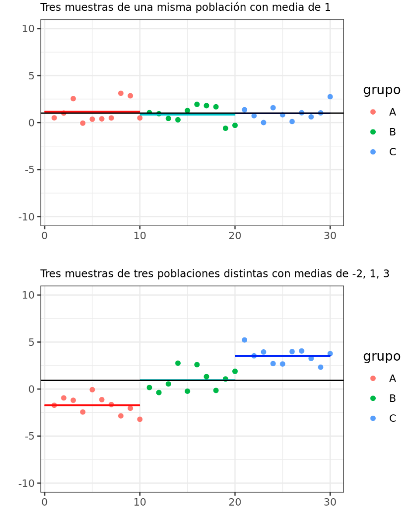
The statistic studied in ANOVA ($F_{ratio}$), is calculated as the ratio between the variance of the means of the groups (between-group variance) and the average of the variance within the groups (within-group variance). This statistic follows an F distribution of Fisher-Snedecor. If the null hypothesis is met, the $F$ statistic acquires the value of 1 since the between-group variance is equal to the within-group variance. As the means of the groups move away from each other, the greater the between-group variance compared to the within-group variance, which generates $F$ values greater than 1, which have a lower associated probability (lower the p-value).
Specifically, if $S_1^2$ is the variance of a sample of size $N_1$ drawn from a normal population of variance $\sigma_1^2$, and $S_2^2$ is the variance of a sample of size $N_2$ drawn from a normal population of variance $\sigma_2^2$, and both samples are independent, the quotient:
$$F = \frac{S_1^2/\sigma_1^2}{S_2^2/\sigma_2^2}$$is distributed as a F of Fisher-Snedecor variable with ($N_1$ and $N_2$) degrees of freedom. In the case of ANOVA, since two of the conditions are the normality of the groups and the homoscedasticity of variance ($\sigma_1^2$ = $\sigma_1^2$), the $F$ value can be obtained by dividing the two variances calculated from the samples (between-group variance and within-group variance).
There are different types of ANOVA depending on whether it is independent data (between-subjects ANOVA), if they are paired (repeated measures ANOVA), if they compare the dependent quantitative variable against the levels of a single qualitative variable or factor (one-way ANOVA) or against two factors (two-way ANOVA). The latter can in turn be additive or interaction (the factors are independent or not). Each of these types of ANOVA has a series of its own requirements.
This document shows how to use the Pingouin library to perform ANOVA analysis in python.
One-way ANOVA for independent data
Definition
One-way ANOVA, also known as single-factor ANOVA or single-factor factorial model, allows us to study whether there are significant differences between the mean of a continuous random variable at the different levels of another qualitative variable or factor, when the data are not paired. It is an extension of the independent t-tests for more than two groups.
The hypotheses tested in a one-way ANOVA are:
$H_0$: There are no differences between the means of the different groups: $\mu_1 = \mu_2 ... = \mu_k = \mu$
$H_1$: At least one pair of means are significantly different from each other.
Another way to state the hypotheses of an ANOVA is as follows: if $\mu$ is considered as the expected value for any observation of the population (the mean of all observations without taking into account the different levels), and $\alpha_i$ is the effect introduced by level $i$. The mean of a certain level ($\mu_i$) can be defined as:
$$\mu_i = \mu + \alpha_i$$$H_0$: No level introduces an effect on the total mean: $\alpha_1 = \alpha_2 =... \alpha_k = 0$
$H_1$: At least one level introduces an effect that shifts its mean: Some $\alpha_i \neq 0$
As mentioned before, the difference between means is detected through the study of the variance between groups and within groups. To achieve this, ANOVA requires a decomposition of the variance based on the following idea:
$$\text{Total variability =}$$$$\text{variability due to the different levels of the factor + residual variability}$$which is equivalent to:
$$\text{variability explained by the factor + variability not explained by the factor}$$which is equivalent to:
$$\text{(variance between levels) + (variance within levels)}$$To be able to calculate the different variances, first the Sums of Squares (SS) must be obtained:
Total sum of squares (TSS): measures the total variability of the data, it is defined as the sum of the squares of the differences of each observation with respect to the general mean of all observations. The degrees of freedom of the total sum of squares are equal to the total number of observations minus one (N-1).
Sum of squares due to treatment (SST): measures the variability in the data associated with the effect of the factor on the mean (the difference of the means between the different levels or groups). It is obtained as the sum of the squares of the deviations of the mean of each group with respect to the general mean, weighting each squared difference by the number of observations of each group. The corresponding degrees of freedom are equal to the number of levels of the factor minus one (k-1).
Sum of squares of errors (SSE): measures the variability within each level, that is, the variability that is not due to the qualitative variable. It is calculated as the sum of the squares of the deviations of each observation with respect to the mean of the level to which it belongs. The degrees of freedom assigned to the sum of residual squares are equivalent to the difference between the total degrees of freedom and the degrees of freedom of the factor, or what is the same (N-k). In statistics, the term error or residual is used since it is considered that this is the variability that the data show due to measurement errors. From a biological point of view, it makes more sense to call it sum of squares within groups since it is known that the observed variability is not only due to measurement errors, but to the many factors that are not controlled and that affect biological processes.
Once the Sum of Squares is decomposed, the decomposition of the variance can be obtained by dividing the Sum of Squares by the respective degrees of freedom. Strictly speaking, the quotient between the Sum of Squares and its corresponding degrees of freedom is called Mean Sum of Squares and can be used as an estimator of the variance:
$\hat{S}_T^2 = \frac{TSS}{N-1} =$ Total Mean Squares = Total Quasi-variance (total sample variance)
$\hat{S}_t^2 = \frac{SST}{k-1} =$ Factor Mean Squares = Between-group variance (variance between the means of the different levels)
$\hat{S}_E^2 = \frac{SSE}{N-k} =$ Error Mean Squares = Within-group variance (variance within the levels, known as residual or error variance)
Note: ANOVA is defined as analysis of variance, but in a strict sense, it is an analysis of the Mean Sum of Squares.
Once the estimation of the variance is decomposed, the $F_{ratio}$ statistic is obtained by dividing the between-group variance by the within-group variance:
$$F_{ratio} = \frac{Factor \ Mean \ Squares}{Error \ Mean \ Squares} = \frac{\hat{S}_t^2}{\hat{S}_E^2} = \frac{between-group \ variance}{within-group \ variance} \sim F_{k-1,N-k}$$Since by definition the $F_{ratio}$ statistic follows a F Fisher-Snedecor distribution with $k-1$ and $N-t$ degrees of freedom, the probability of obtaining values equal to or more extreme than those observed (p-values) can be known.
Conditions for one-way ANOVA with independent data
The conditions for a one-way ANOVA with independent data are:
Independence: the observations must be random and independent of each other. The groups (levels of the factor) must be independent of each other.
Normal distribution of each of the levels or groups: the variable under study must be normally distributed in each of the groups, this condition being less strict the larger the size of each group. The best way to verify normality is to study the residuals of each observation with respect to the mean of the group to which they belong.
Although ANOVA is quite robust even when there is a certain lack of normality, if the symmetry is very pronounced and the size of each group is not very large, the non-parametric Kruskal-Wallis H test can be used instead. It is often recommended to stick with ANOVA unless the lack of normality is very extreme.
Atypically extreme data can completely invalidate the conclusions of an ANOVA. If extreme residuals are observed, it is necessary to study in detail which observations they belong to, and it is advisable to recalculate the ANOVA without them and compare the results obtained.
Same variance between groups (homoscedasticity): the variance within the groups must be approximately equal in all of them. This is because in the null hypothesis it is considered that all observations come from the same population, so they have the same mean and also the same variance.
This condition is more important the smaller the size of the groups.
ANOVA is quite robust to the lack of homoscedasticity if the design is balanced (same number of observations per group).
In unbalanced designs, the lack of homoscedasticity has a greater impact. If the smaller groups are the ones with the highest variance, the number of false positives will increase. If, on the other hand, the larger groups have a higher variance, the false negatives will increase.
When homoscedasticity cannot be accepted, a heteroscedastic ANOVA can be used, which uses the Welch correction (Welch test).
In the book Handbook of Biological Statistics it is considered highly advisable to use balanced designs. This being the case, they consider ANOVA reliable as long as the number of observations per group is not less than 10 and the standard deviation does not vary more than 3 times between groups. For unbalanced models, they recommend examining homoscedasticity in detail, if the variances of the groups are not very similar, it is better to use Welch's ANOVA.
Multiple comparison of means. POST-HOC contrasts
If an ANOVA is significant, it means that at least two of the compared means are significantly different from each other, but it does not determine which ones. To identify them, the means of all groups must be compared two by two using a t-test or another test that allows comparing 2 groups. This is known as post-hoc analysis. Due to the inflation of the type I error, the more comparisons are made, the greater the probability of finding significant differences. For example, for a significance level $\alpha$ = 0.05, 5 significant comparisons are expected out of every 100 just by chance.
To avoid this problem, the significance level can be adjusted based on the number of comparisons (significance correction). If no correction is made, the possibility of false positives (type I error) increases, but if the corrections are very strict, differences that are actually significant may be considered non-significant (type II error). The need for correction or not, and of what type, must be studied carefully in each case. The main post-hoc comparison methods are described below:
Fisher's LSD intervals (Least Significance Method)
Being $\overline{x}_i$ the sample mean of a group, the estimated standard deviation of said mean (assuming the homoscedasticity of the groups) is equal to the square root of the Mean Squares of the Error, which as seen in previous sections, is the estimation of the within-group variance divided by the number of observations of said group. Also assuming the normality of the groups, the LSD interval can be obtained as:
$$\overline{x}_i \pm \frac{\sqrt{2}}{2}t^{\alpha}_{gl(error)}\sqrt{\frac{SSE}{n}}$$The LSD intervals are basically a set of individual t-tests with the only difference that, instead of calculating a pooled SD using only the two compared groups, it calculates the pooled SD from all available groups.
The further the intervals of two groups are, the more different their means are, with the difference being significant if the intervals do not overlap. It is important to understand that the LSD intervals are used to compare the means but cannot be interpreted as a confidence interval. The LSD method does not involve any type of significance correction, which is why its use seems to be discouraged for determining significance, although it is useful for identifying which groups have the most distant means.
Bonferroni adjustment
This is possibly the most widespread significance adjustment, although it is not recommended for most practical situations. The Bonferroni correction consists of dividing the significance level $\alpha$ by the number of pairwise comparisons made.
$$\alpha_{corrected} = \frac{\alpha}{number \ of \ groups}$$With this correction, it is ensured that the probability of obtaining at least one false positive among all comparisons (family-wise error rate) is $\leq \alpha$. It allows testing a general null hypothesis (that all tested null hypotheses are true) simultaneously, which is rarely of interest in research. It is considered an excessively conservative method, especially as the number of comparisons increases. Its use is discouraged except in very specific situations. False discovery rate control is a recommended alternative to Bonferroni-type adjustments in health studies, Mark E. Glickman.
Holm–Bonferroni Adjustment
With this method, the significance value $\alpha$ is corrected sequentially, making it less conservative than the Bonferroni method. Even so, it is also not usually recommended if more than 6 comparisons are made.
The process consists of performing a t-test for all comparisons and ordering them from lowest to highest p-value. The significance level for the first comparison (the one with the lowest p-value) is corrected by dividing $\alpha$ by the total number of comparisons. If after the correction it is not significant, the process is stopped. If it is, the significance level of the next comparison (second lowest p-value) is corrected by dividing by the number of comparisons minus one. The process is repeated until it stops when the comparison is no longer significant.
Tukey-Kramer Honest Significant Difference (HSD)
This is the recommended adjustment when the number of groups to compare is greater than 6 and the design is balanced (same number of observations per group). In the case of unbalanced models, the HSD method is conservative, requiring large differences to be significant.
The Tukey's test is very similar to a t-test, except that it corrects the experiment wise error rate. It achieves this by using a statistic that follows a distribution called the studentized range distribution instead of a t-distribution. This statistic is defined as:
$$q_{calculated} = \frac{\overline{x}_{max}-\overline{x}_{min}}{S\sqrt{2/n}}$$where $\overline{x}_{max}$ is the larger of the means of the two compared groups, $\overline{x}_{min}$ is the smaller, S is the pooled SD of these two groups, and n is the total number of observations in the two groups.
For each pair of groups, the $q_{calculated}$ value is obtained and compared with the expected value according to a studentized range distribution with the corresponding degrees of freedom. If the probability is less than the established significance level $\alpha$, the difference in means is considered significant. As with the LSD intervals, it is possible to calculate HSD intervals to study their overlap.
Dunnett’s correction (Dunnett’s test)
This is the equivalent of the Tukey-Kramer (HSD) test recommended when, instead of comparing all groups with each other ($\frac{(k-1)k}{2}$ comparisons), you only want to compare them against a control group ($k-1$ comparisons). It is frequently used in medical experiments.
Disadvantages of controlling the false positive rate using Bonferroni
As seen in the examples, when making multiple comparisons, it is important to control for the inflation of type I error. However, corrections like Bonferroni or similar ones have a series of problems.
The first problem is that the method was developed to test the universal null hypothesis that the two groups are equal for all tested variables, not to apply it individually to each test. For example, suppose a researcher wants to determine if a new teaching method is effective using students from 20 schools. In each school, a control group and a group subjected to the new method are randomly selected, and a statistical test is performed between them considering a significance level of $\alpha = 0.05$. The Bonferroni correction involves comparing the p-value obtained in the 20 tests against 0.05/20 = 0.0025. If any of the p-values is significant, the Bonferroni conclusion is that the null hypothesis that the new teaching system is not effective in all groups (schools) is rejected, so it can be affirmed that the teaching method is effective for some of the 20 groups, but not which ones or how many. This type of information is not of interest in the vast majority of studies, since what is desired is to know which groups differ.
The second problem with the Bonferroni correction is that the same comparison is interpreted differently depending on the number of tests performed. Suppose a researcher performs 20 hypothesis tests and all of them result in a p-value of 0.001. Applying the Bonferroni correction, if the significance limit for an individual test is $\alpha=0.05$, the corrected significance level turns out to be 0.05/20 = 0.0025, so the researcher concludes that all tests are significant. A second researcher reproduces the same analyses in another laboratory and obtains the same results, but to confirm them even more, he performs 80 additional statistical tests. This time, his corrected significance level becomes 0.05/100 = 0.0005. Now, none of the tests can be considered significant, so due to the increase in the number of contrasts, the conclusions are completely opposite.
Given the problems involved, what is the Bonferroni correction for?
The fact that its application in some disciplines is not appropriate does not mean that it cannot be in other areas. Imagine a factory that produces light bulbs in batches of 1000 units and that testing each one before distributing them is not feasible. An alternative is to check only a sample from each batch, rejecting any batch that has more than x defective bulbs in the sample. Of course, the decision may be wrong for a given batch, but according to the Neyman-Pearson theory, the value of x can be found for which the error rate is minimized. However, the probability of finding x defective bulbs in the sample depends on the size of the sample, or in other words, on the number of tests performed per batch. If the size is increased, so does the probability of rejecting the batch, and this is where the Bonferroni correction recalculates the value of x that keeps the error rate minimized.
False Discovery Rate (FDR), Benjamini & Hochberg (BH)
The methods described above focus on correcting the inflation of type I error (false positive rate), that is, the probability of rejecting the null hypothesis when it is true. This approach is useful when a limited number of comparisons are used. For large-scale multiple testing scenarios such as genomic studies, where thousands of tests are performed simultaneously, the result of these methods is too conservative and prevents the detection of real differences. An alternative is to control the false discovery rate.
The false discovery rate (FDR) is defined as: (all definitions are equivalent)
The expected proportion of tests in which the null hypothesis is true, among all tests that have been considered significant.
FDR is the probability that a null hypothesis is true having been rejected by the statistical test.
Among all tests considered significant, the FDR is the expected proportion of those tests for which the null hypothesis is true.
It is the proportion of significant tests that are not really significant.
The expected proportion of false positives among all tests considered significant.
The objective of controlling the false discovery rate is to establish a significance limit for a set of tests such that, among all tests considered significant, the proportion of true null hypotheses (false positives) does not exceed a certain value. Another added advantage is its easy interpretation, for example, if a study publishes statistically significant results for an FDR of 10%, the reader is assured that at most 10% of the results considered significant are false positives.
When a researcher uses a significance level $\alpha$, for example of 0.05, they usually expect some certainty that only a small fraction of the significant tests correspond to true null hypotheses (false positives). However, this does not have to be the case, since the latter depends on the frequency with which the tested null hypothesis is actually true. An extreme case would be one in which all null hypotheses are actually true, in which case, 100% of the tests that on average are significant are false positives. Therefore, the proportion of false positives (false discovery rate) depends on the number of null hypotheses that are true among all the contrasts.
Exploratory analyses in which the researcher tries to identify significant results with little prior knowledge are characterized by a high proportion of false null hypotheses. Analyses that are done to confirm hypotheses, in which the design has been oriented based on prior knowledge, usually have a high proportion of true null hypotheses. Ideally, if the proportion of true null hypotheses among all contrasts were known beforehand, the appropriate significance limit could be precisely adjusted for each scenario, however, this does not happen in reality.
The first approach to control the false discovery rate was described by Benjamini and Hochberg in 1995. According to their publication, if you want to ensure that in a study with n comparisons the false discovery rate does not exceed a percentage d, you must:
Order the n tests from lowest to highest p-value ($p_1, \ p_2, \ ... \ p_n$)
Define k as the last position for which it is true that $p_i \leq d \frac{i}{n}$
Consider all p-values up to position k ($p_1, \ p_2, \ ... \ p_k$) as significant
The main advantage of controlling the false discovery rate becomes more apparent the more comparisons are made, for this reason it is usually used in situations with hundreds or thousands of comparisons. However, the method can also be applied to smaller studies.
The method proposed by Benjamini & Hochberg assumes, when estimating the number of null hypotheses erroneously considered false, that all null hypotheses are true. As a consequence, the estimation of the FDR is inflated and therefore conservative. For more detailed information on multiple comparisons, see the document: Multiple comparisons: p-value correction and FDR.
Effect size $\eta^2$
The effect size of an ANOVA is the value that allows measuring how much variance in the dependent variable is the result of the influence of the independent qualitative variable, or what is the same, how much the independent variable (factor) affects the dependent variable. In ANOVA, the most used measure of effect size is $\eta^2$ which is defined as:
$$\eta^2= \frac{Suma Cuadrados_{entre \ grupos}}{Suma Cuadrados_{total}}$$The most used classification levels for the effect size are:
0.01 = small
0.06 = medium
0.14 = large
Power of one-way ANOVA
Power tests allow determining the probability of finding significant differences between the means for a given $\alpha$ indicating the size of the groups, or calculating the size that the groups must have to be able to detect with a certain probability a difference in the means if it exists. In those cases where you want to know the size that the samples must have, it is necessary to know (either from previous experiments or from pilot samples) an estimate of the population variance.
Results of an ANOVA
When communicating the results of an ANOVA, it is convenient to indicate the value obtained for the $F$ statistic, the degrees of freedom, the p-value, and the effect size ($\eta^2$).
It may happen that an ANOVA analysis indicates that there are significant differences between the means and then the t-tests do not find any comparison that is significant. This is not contradictory, it is simply because they are two different techniques.
Example
Suppose a study wants to check if there is a significant difference between the % of successful hits of baseball players depending on the position they play. If there is, we want to know which positions differ from the rest.
Libraries
The libraries used in this example are:
# ==============================================================================
# Libraries
# ==============================================================================
import pandas as pd
import numpy as np
import matplotlib.pyplot as plt
plt.style.use('fivethirtyeight')
plt.rcParams['lines.linewidth'] = 1.5
plt.rcParams['font.size'] = 8
import seaborn as sns
import pingouin as pg
from statsmodels.graphics.factorplots import interaction_plot
Data
The following table contains a sample of randomly selected league players.
position = ["OF", "IF", "IF", "OF", "IF", "IF", "OF", "OF", "IF", "IF", "OF",
"OF", "IF", "OF", "IF", "IF", "IF", "OF", "IF", "OF", "IF", "OF",
"IF", "OF", "IF", "DH", "IF", "IF", "IF", "OF", "IF", "IF", "IF",
"IF", "OF", "IF", "OF", "IF", "IF", "IF", "IF", "OF", "OF", "IF",
"OF", "OF", "IF", "IF", "OF", "OF", "IF", "OF", "OF", "OF", "IF",
"DH", "OF", "OF", "OF", "IF", "IF", "IF", "IF", "OF", "IF", "IF",
"OF", "IF", "IF", "IF", "OF", "IF", "IF", "OF", "IF", "IF", "IF",
"IF", "IF", "IF", "OF", "DH", "OF", "OF", "IF", "IF", "IF", "OF",
"IF", "OF", "IF", "IF", "IF", "IF", "OF", "OF", "OF", "DH", "OF",
"IF", "IF", "OF", "OF", "C", "IF", "OF", "OF", "IF", "OF", "IF",
"IF", "IF", "OF", "C", "OF", "IF", "C", "OF", "IF", "DH", "C", "OF",
"OF", "IF", "C", "IF", "IF", "IF", "IF", "IF", "IF", "OF", "C", "IF",
"OF", "OF", "IF", "OF", "IF", "OF", "DH", "C", "IF", "OF", "IF",
"IF", "OF", "IF", "OF", "IF", "C", "IF", "IF", "OF", "IF", "IF",
"IF", "OF", "OF", "OF", "IF", "IF", "C", "IF", "C", "C", "OF", "OF",
"OF", "IF", "OF", "IF", "C", "DH", "DH", "C", "OF", "IF", "OF", "IF",
"IF", "IF", "C", "IF", "OF", "DH", "IF", "IF", "IF", "OF", "OF", "C",
"OF", "OF", "IF", "IF", "OF", "OF", "OF", "OF", "OF", "OF", "IF",
"IF", "DH", "OF", "IF", "IF", "OF", "IF", "IF", "IF", "IF", "OF",
"IF", "C", "IF", "IF", "C", "IF", "OF", "IF", "DH", "C", "OF", "C",
"IF", "IF", "OF", "C", "IF", "IF", "IF", "C", "C", "C", "OF", "OF",
"IF", "IF", "IF", "IF", "OF", "OF", "C", "IF", "IF", "OF", "C", "OF",
"OF", "OF", "OF", "OF", "OF", "OF", "OF", "OF", "OF", "OF", "C",
"IF", "DH", "IF", "C", "DH", "C", "IF", "C", "OF", "C", "C", "IF",
"OF", "IF", "IF", "IF", "IF", "IF", "IF", "IF", "IF", "OF", "OF",
"OF", "IF", "OF", "OF", "IF", "IF", "IF", "OF", "C", "IF", "IF",
"IF", "IF", "OF", "OF", "IF", "OF", "IF", "OF", "OF", "OF", "IF",
"OF", "OF", "IF", "OF", "IF", "C", "IF", "IF", "C", "DH", "OF", "IF",
"C", "C", "IF", "C", "IF", "OF", "C", "C", "OF"]
batting = [0.359, 0.34, 0.33, 0.341, 0.366, 0.333, 0.37, 0.331, 0.381, 0.332,
0.365, 0.345, 0.313, 0.325, 0.327, 0.337, 0.336, 0.291, 0.34, 0.31,
0.365, 0.356, 0.35, 0.39, 0.388, 0.345, 0.27, 0.306, 0.393, 0.331,
0.365, 0.369, 0.342, 0.329, 0.376, 0.414, 0.327, 0.354, 0.321, 0.37,
0.313, 0.341, 0.325, 0.312, 0.346, 0.34, 0.401, 0.372, 0.352, 0.354,
0.341, 0.365, 0.333, 0.378, 0.385, 0.287, 0.303, 0.334, 0.359, 0.352,
0.321, 0.323, 0.302, 0.349, 0.32, 0.356, 0.34, 0.393, 0.288, 0.339,
0.388, 0.283, 0.311, 0.401, 0.353, 0.42, 0.393, 0.347, 0.424, 0.378,
0.346, 0.355, 0.322, 0.341, 0.306, 0.329, 0.271, 0.32, 0.308, 0.322,
0.388, 0.351, 0.341, 0.31, 0.393, 0.411, 0.323, 0.37, 0.364, 0.321,
0.351, 0.329, 0.327, 0.402, 0.32, 0.353, 0.319, 0.319, 0.343, 0.288,
0.32, 0.338, 0.322, 0.303, 0.356, 0.303, 0.351, 0.325, 0.325, 0.361,
0.375, 0.341, 0.383, 0.328, 0.3, 0.277, 0.359, 0.358, 0.381, 0.324,
0.293, 0.324, 0.329, 0.294, 0.32, 0.361, 0.347, 0.317, 0.316, 0.342,
0.368, 0.319, 0.317, 0.302, 0.321, 0.336, 0.347, 0.279, 0.309, 0.358,
0.318, 0.342, 0.299, 0.332, 0.349, 0.387, 0.335, 0.358, 0.312, 0.307,
0.28, 0.344, 0.314, 0.24, 0.331, 0.357, 0.346, 0.351, 0.293, 0.308,
0.374, 0.362, 0.294, 0.314, 0.374, 0.315, 0.324, 0.382, 0.353, 0.305,
0.338, 0.366, 0.357, 0.326, 0.332, 0.323, 0.306, 0.31, 0.31, 0.333,
0.34, 0.4, 0.389, 0.308, 0.411, 0.278, 0.326, 0.335, 0.316, 0.371,
0.314, 0.384, 0.379, 0.32, 0.395, 0.347, 0.307, 0.326, 0.316, 0.341,
0.308, 0.327, 0.337, 0.36, 0.32, 0.372, 0.306, 0.305, 0.347, 0.281,
0.281, 0.296, 0.306, 0.343, 0.378, 0.393, 0.337, 0.327, 0.336, 0.32,
0.381, 0.306, 0.358, 0.311, 0.284, 0.364, 0.315, 0.342, 0.367, 0.307,
0.351, 0.372, 0.304, 0.296, 0.332, 0.312, 0.437, 0.295, 0.316, 0.298,
0.302, 0.342, 0.364, 0.304, 0.295, 0.305, 0.359, 0.335, 0.338, 0.341,
0.3, 0.378, 0.412, 0.273, 0.308, 0.309, 0.263, 0.291, 0.359, 0.352,
0.262, 0.274, 0.334, 0.343, 0.267, 0.321, 0.3, 0.327, 0.313, 0.316,
0.337, 0.268, 0.342, 0.292, 0.39, 0.332, 0.315, 0.298, 0.298, 0.331,
0.361, 0.272, 0.287, 0.34, 0.317, 0.327, 0.354, 0.317, 0.311, 0.174,
0.302, 0.302, 0.291, 0.29, 0.268, 0.352, 0.341, 0.265, 0.307, 0.36,
0.305, 0.254, 0.279, 0.321, 0.305, 0.35, 0.308, 0.326, 0.219, 0.23,
0.322, 0.405, 0.321, 0.291, 0.312, 0.357, 0.324]
data = pd.DataFrame({'position': position, 'batting': batting})
data.head(4)
| position | batting | |
|---|---|---|
| 0 | OF | 0.359 |
| 1 | IF | 0.340 |
| 2 | IF | 0.330 |
| 3 | OF | 0.341 |
Number of groups, observations per group and distribution of observations
The number of groups and the number of observations per group are identified to determine if it is a balanced model. The mean and standard deviation of each group are also calculated.
# Number of observations per group
# ==============================================================================
data.groupby('position').size()
position C 39 DH 14 IF 154 OF 120 dtype: int64
# Mean and standard deviation per group
# ==============================================================================
data.groupby('position').agg(['mean', 'std'])
| batting | ||
|---|---|---|
| mean | std | |
| position | ||
| C | 0.322615 | 0.045132 |
| DH | 0.347786 | 0.036037 |
| IF | 0.331526 | 0.037095 |
| OF | 0.334250 | 0.029444 |
Since the number of observations per group is not constant, it is an unbalanced model. It is important to keep this in mind when checking the conditions of normality and homoscedasticity.
Graphical analysis
Two of the most useful representations before performing an ANOVA are the Box-Plot and Violin-Plot graphs.
fig, ax = plt.subplots(1, 1, figsize=(8, 4))
sns.boxplot(x="position", y="batting", data=data, ax=ax)
sns.swarmplot(x="position", y="batting", data=data, color='black', alpha = 0.5, ax=ax);

This type of representation allows for a preliminary identification of asymmetries, outliers, or differences in variances. In this case, the 4 groups seem to follow a symmetrical distribution. At the IF level, some extreme values are detected that will need to be studied in detail in case they need to be removed. The size of the boxes is similar for all levels, so there are no signs of lack of homoscedasticity.
Verify conditions for an ANOVA
Independence
The groups (categorical variable) and players within each group are independent of each other since a random sampling of players from the entire league (not just from the same team) has been done.
Normal distribution of observations
The quantitative variable must be normally distributed in each of the groups. The study of normality can be done graphically (qqplot) or with hypothesis tests.
# qqplot graphs
# ==============================================================================
fig, axs = plt.subplots(2, 2, figsize=(8, 7))
pg.qqplot(data.loc[data.position=='OF', 'batting'], dist='norm', ax=axs[0,0])
axs[0,0].set_title('OF')
pg.qqplot(data.loc[data.position=='IF', 'batting'], dist='norm', ax=axs[0,1])
axs[0,1].set_title('IF')
pg.qqplot(data.loc[data.position=='DH', 'batting'], dist='norm', ax=axs[1,0])
axs[1,0].set_title('DH')
pg.qqplot(data.loc[data.position=='C', 'batting'], dist='norm', ax=axs[1,1])
axs[1,1].set_title('C')
plt.tight_layout()

# Shapiro-Wilk normality test
# ==============================================================================
pg.normality(data=data, dv='batting', group='position')
| W | pval | normal | |
|---|---|---|---|
| position | |||
| OF | 0.993361 | 0.842244 | True |
| IF | 0.974849 | 0.006406 | False |
| DH | 0.972155 | 0.904090 | True |
| C | 0.980154 | 0.709178 | True |
Neither the graphical analysis nor the hypothesis tests show evidence of lack of normality.
Constant variance between groups (homoscedasticity)
Since there is an IF group that is on the limit to accept that it is normally distributed, the Levene test is more appropriate than the Bartlett test.
# Homoscedasticity test
# ==============================================================================
pg.homoscedasticity(data=data, dv='batting', group='position', method='levene')
| W | pval | equal_var | |
|---|---|---|---|
| levene | 2.605659 | 0.051799 | True |
According to the Levene test, there is no significant evidence to indicate a lack of homoscedasticity.
ANOVA Test
# One-way ANOVA test
# ==============================================================================
pg.anova(data=data, dv='batting', between='position', detailed=True)
| Source | SS | DF | MS | F | p-unc | np2 | |
|---|---|---|---|---|---|---|---|
| 0 | position | 0.007557 | 3 | 0.002519 | 1.994349 | 0.114693 | 0.018186 |
| 1 | Within | 0.407984 | 323 | 0.001263 | NaN | NaN | NaN |
A p-value greater than 0.1 is very weak evidence against the null hypothesis that all groups have the same mean. The eta-squared value ($\eta^2$) is 0.018, which can be considered a small effect size.
Post-hoc multiple comparisons
In this case, the ANOVA was not significant, so it makes no sense to perform pairwise comparisons. However, for educational purposes, it is shown how to obtain the TukeyHSD tests.
# Post-hoc Tukey test
# ==============================================================================
pg.pairwise_tukey(data=data, dv='batting', between='position').round(3)
| A | B | mean(A) | mean(B) | diff | se | T | p-tukey | hedges | |
|---|---|---|---|---|---|---|---|---|---|
| 0 | C | DH | 0.323 | 0.348 | -0.025 | 0.011 | -2.273 | 0.106 | -0.577 |
| 1 | C | IF | 0.323 | 0.332 | -0.009 | 0.006 | -1.399 | 0.501 | -0.229 |
| 2 | C | OF | 0.323 | 0.334 | -0.012 | 0.007 | -1.776 | 0.287 | -0.341 |
| 3 | DH | IF | 0.348 | 0.332 | 0.016 | 0.010 | 1.639 | 0.358 | 0.437 |
| 4 | DH | OF | 0.348 | 0.334 | 0.014 | 0.010 | 1.349 | 0.533 | 0.446 |
| 5 | IF | OF | 0.332 | 0.334 | -0.003 | 0.004 | -0.629 | 0.923 | -0.080 |
As expected, no significant difference is found between any pair of means.
Conclusion
In the study carried out, a small effect size was observed and the ANOVA inference techniques have not found statistical significance to reject that the means are equal among all groups.
Two-way ANOVA for independent data
Definition
The two-way analysis of variance, also known as a factorial plan with two factors, is used to study the relationship between a quantitative dependent variable and two qualitative independent variables (factors), each with several levels. The two-way ANOVA allows studying how each of the factors influences the dependent variable by themselves (additive model) as well as the influence of the combinations that can occur between them (model with interaction).
Suppose we want to study the effect of a drug on blood pressure (quantitative dependent variable) depending on the patient's sex (levels: male, female) and age group (levels: child, adult, elderly).
The simple effect of the factors consists of studying how the effect of the drug varies depending on sex without differentiating by age, as well as studying how the effect of the drug varies depending on age without taking sex into account. The effect of the double interaction consists of studying whether the influence of one of the factors varies depending on the levels of the other factor. That is, if the influence of the sex factor on the activity of the drug is different depending on the age of the patient or, what is the same, if the activity of the drug for a certain age is different depending on whether you are a man or a woman.
Conditions for two-way ANOVA for independent data
The necessary conditions for a two-way ANOVA to be valid, as well as the process to follow to perform it, are similar to the one-way ANOVA. The only differences are:
Hypothesis: the two-way ANOVA with repetitions combines 3 null hypotheses: that the means of the observations grouped by one factor are equal, that the means of the observations grouped by the other factor are equal, and that there is no interaction between the two factors.
It requires calculating the Sum of Squares and Mean Squares for both factors. It is common to find that one factor is called "treatment" and the other block.
It is important to keep in mind that the order in which the factors are multiplied does not affect the result of the ANOVA only if the size of the groups is equal (balanced model), otherwise it does matter. For this reason, it is recommended that the design be balanced.
In addition, the study of the interaction of the two factors is only possible if there are several observations for each of the combinations of the levels.
Effect size
In the case of ANOVA with two factors, the eta-squared ($\eta^2$) effect size can be calculated for each of the two factors as well as for the interaction.
Example 1
A construction materials company wants to study the influence of thickness and type of tempering on the maximum strength of steel sheets. To do this, they measure the stress to failure (quantitative dependent variable) for two types of tempering (slow and fast) and three sheet thicknesses (8mm, 16mm, and 24mm).
Note: in order to simplify the example, it is assumed that the conditions for a two-way ANOVA are met. In a real case, the conditions on which a method or technique is based must always be validated.
Libraries
The libraries used in this example are:
import pandas as pd
import numpy as np
import matplotlib.pyplot as plt
import seaborn as sns
import pingouin as pg
Data
strength = [15.29, 15.89, 16.02, 16.56, 15.46, 16.91, 16.99, 17.27, 16.85,
16.35, 17.23, 17.81, 17.74, 18.02, 18.37, 12.07, 12.42, 12.73,
13.02, 12.05, 12.92, 13.01, 12.21, 13.49, 14.01, 13.30, 12.82,
12.49, 13.55, 14.53]
tempering = ["fast"] * 15 + ["slow"] * 15
thickness = ([8] * 5 + [16] * 5 + [24] * 5) * 2
data = pd.DataFrame({
'tempering': tempering,
'thickness': thickness,
'strength': strength
})
data.head()
| tempering | thickness | strength | |
|---|---|---|---|
| 0 | fast | 8 | 15.29 |
| 1 | fast | 8 | 15.89 |
| 2 | fast | 8 | 16.02 |
| 3 | fast | 8 | 16.56 |
| 4 | fast | 8 | 15.46 |
Descriptive and graphical analysis
First, Box-plot diagrams are generated to identify possible notable differences, asymmetries, outliers, and homogeneity of variance between the different levels. The mean and variance of each group are also calculated.
fig, axs = plt.subplots(1, 2, figsize=(10, 4))
axs[0].set_title('Strength vs tempering')
sns.boxplot(x="tempering", y="strength", data=data, ax=axs[0])
sns.swarmplot(x="tempering", y="strength", data=data, color='black',
alpha = 0.5, ax=axs[0])
axs[1].set_title('Strength vs thickness')
sns.boxplot(x="thickness", y="strength", data=data, ax=axs[1])
sns.swarmplot(x="thickness", y="strength", data=data, color='black',
alpha = 0.5, ax=axs[1]);

fig, ax = plt.subplots(1, 1, figsize=(8, 4))
ax.set_title('Strength vs tempering and thickness')
sns.boxplot(x="tempering", y="strength", hue='thickness', data=data, ax=ax);

print('Mean strength and standard deviation by tempering')
data.groupby('tempering')['strength'].agg(['mean', 'std'])
Mean strength and standard deviation by tempering
| mean | std | |
|---|---|---|
| tempering | ||
| fast | 16.850667 | 0.927643 |
| slow | 12.974667 | 0.711345 |
print('Mean strength and standard deviation by thickness')
data.groupby('thickness')['strength'].agg(['mean', 'std'])
Mean strength and standard deviation by thickness
| mean | std | |
|---|---|---|
| thickness | ||
| 8 | 14.151 | 1.836993 |
| 16 | 15.001 | 2.036797 |
| 24 | 15.586 | 2.442354 |
print('Mean strength and standard deviation by tempering and thickness')
data.groupby(['tempering', 'thickness'])['strength'].agg(['mean', 'std'])
Mean strength and standard deviation by tempering and thickness
| mean | std | ||
|---|---|---|---|
| tempering | thickness | ||
| fast | 8 | 15.844 | 0.500030 |
| 16 | 16.874 | 0.334186 | |
| 24 | 17.834 | 0.417169 | |
| slow | 8 | 12.458 | 0.420797 |
| 16 | 13.128 | 0.672473 | |
| 24 | 13.338 | 0.783371 |
From the graphical representation and the calculation of the means, it can be inferred that there is a difference in the strength achieved depending on the type of tempering. The strength seems to increase as the thickness of the sheet increases, although it is not clear that the difference in the means is significant. The distribution of the observations of each level seems symmetrical without the presence of outliers. A priori, it seems that the necessary conditions for an ANOVA are met.
Another way to graphically identify possible interactions between the two factors is through what are known as "interaction plots". If the lines that describe the data for each of the levels are parallel, it means that the behavior is similar regardless of the level of the factor, that is, there is no interaction.
fig, ax = plt.subplots(figsize=(6, 4))
fig = interaction_plot(
x = data.tempering,
trace = data.thickness,
response = data.strength,
ax = ax,
)

fig, ax = plt.subplots(figsize=(6, 4))
fig = interaction_plot(
x = data.thickness,
trace = data.tempering,
response = data.strength,
ax = ax,
)

The first interaction plot seems to indicate that the increase in strength between the two types of tempering is proportional for the three thicknesses. In the second plot, a certain deviation is observed in the 24mm thickness. This could be due to simple variability or because there is an interaction between the thickness and tempering variables. These indications will be confirmed or discarded by the ANOVA.
ANOVA Test
# Two-way ANOVA test
# ==============================================================================
pg.anova(
data = data,
dv = 'strength',
between = ['tempering', 'thickness'],
detailed = True
).round(4)
| Source | SS | DF | MS | F | p-unc | np2 | |
|---|---|---|---|---|---|---|---|
| 0 | tempering | 112.6753 | 1 | 112.6753 | 380.0820 | 0.0000 | 0.9406 |
| 1 | thickness | 10.4132 | 2 | 5.2066 | 17.5631 | 0.0000 | 0.5941 |
| 2 | tempering * thickness | 1.6035 | 2 | 0.8018 | 2.7045 | 0.0873 | 0.1839 |
| 3 | Residual | 7.1148 | 24 | 0.2964 | NaN | NaN | NaN |
The analysis of variance confirms that there is a significant influence on the strength of the sheets by both factors (tempering and thickness) with large and medium $\eta^2$ effect sizes, respectively. However, no significant interaction between them is detected.
Example 2
Suppose a clinical study analyzes the effectiveness of a drug taking into account two factors, sex (male and female) and youth (young, adult). We want to analyze if the effect is different between any of the levels of each variable by itself or in combination.
This study involves checking if the average effect of the drug is significantly different between any of the following groups: men, women, young people, adults, young men, adult men, young women, and adult women.
Libraries
The libraries used in this example are:
import pandas as pd
import numpy as np
import matplotlib.pyplot as plt
import seaborn as sns
import pingouin as pg
Data
subject = [1, 2, 3, 4, 5, 6, 7, 8, 9, 10, 11, 12, 13, 14, 15, 16, 17, 18, 19, 20,
21, 22, 23, 24, 25, 26, 27, 28, 29, 30]
sex = ["female", "male", "male", "female", "male", "male", "male", "female",
"female", "male", "male", "male", "male", "female", "female", "female",
"male", "female", "female", "male", "male", "female", "male", "male",
"male", "male", "male", "male", "female", "male"]
age = ["adult", "adult", "adult", "adult", "adult", "adult", "young", "young",
"adult", "young", "young", "adult", "young", "young", "young", "adult",
"young", "adult", "young", "young", "young", "young", "adult", "young",
"young", "young", "young", "young", "young", "adult"]
result = [7.1, 11.0, 5.8, 8.8, 8.6, 8.0, 3.0, 5.2, 3.4, 4.0, 5.3, 11.3, 4.6, 6.4,
13.5, 4.7, 5.1, 7.3, 9.5, 5.4, 3.7, 6.2, 10.0, 1.7, 2.9, 3.2, 4.7, 4.9,
9.8, 9.4]
data = pd.DataFrame({
'subject': subject,
'sex': sex,
'age': age,
'result': result
})
data.head()
| subject | sex | age | result | |
|---|---|---|---|---|
| 0 | 1 | female | adult | 7.1 |
| 1 | 2 | male | adult | 11.0 |
| 2 | 3 | male | adult | 5.8 |
| 3 | 4 | female | adult | 8.8 |
| 4 | 5 | male | adult | 8.6 |
Descriptive and graphical analysis
First, Box-plot diagrams are generated to identify possible notable differences, asymmetries, outliers, and homogeneity of variance between the different levels. The mean and variance of each group are also calculated.
fig, axs = plt.subplots(1, 2, figsize=(10, 4))
axs[0].set_title('Results vs age')
sns.boxplot(x="age", y="result", data=data, ax=axs[0])
sns.swarmplot(x="age", y="result", data=data, color='black',
alpha = 0.5, ax=axs[0])
axs[1].set_title('Results vs sex')
sns.boxplot(x="sex", y="result", data=data, ax=axs[1])
sns.swarmplot(x="sex", y="result", data=data, color='black',
alpha = 0.5, ax=axs[1]);

fig, ax = plt.subplots(1, 1, figsize=(8, 4))
ax.set_title('Results vs sex and age')
sns.boxplot(x="age", y="result", hue='sex', data=data, ax=ax);

print('Mean results and standard deviation by age')
data.groupby('age')['result'].agg(['mean', 'std'])
Mean results and standard deviation by age
| mean | std | |
|---|---|---|
| age | ||
| adult | 7.950000 | 2.431049 |
| young | 5.505556 | 2.871047 |
print('Mean results and standard deviation by sex')
data.groupby('sex')['result'].agg(['mean', 'std'])
Mean results and standard deviation by sex
| mean | std | |
|---|---|---|
| sex | ||
| female | 7.445455 | 2.828202 |
| male | 5.926316 | 2.906858 |
print('Mean results and standard deviation by age and sex')
data.groupby(['age', 'sex'])['result'].agg(['mean', 'std'])
Mean results and standard deviation by age and sex
| mean | std | ||
|---|---|---|---|
| age | sex | ||
| adult | female | 6.260000 | 2.170944 |
| male | 9.157143 | 1.900752 | |
| young | female | 8.433333 | 3.106552 |
| male | 4.041667 | 1.157158 |
From the graphical representation and the calculation of the means, it can be inferred that there is a difference in the effect of the drug depending on age and also on sex. The effect seems to be greater in women than in men and in adults than in young people, although the significance will have to be confirmed with the ANOVA. The distribution of the observations of each level seems symmetrical with the presence of a single outlier. A priori, it seems that the necessary conditions for an ANOVA are met, although they will have to be confirmed by studying the residuals.
# Interaction plot
# ==============================================================================
fig, ax = plt.subplots(figsize=(6, 4))
fig = interaction_plot(
x = data.age,
trace = data.sex,
response = data.result,
ax = ax,
)

A clear interaction between both factors is observed. The response to the drug is different between adults and young people, and has an inverse trend depending on sex. In women, the response is greater when they are young than when they are adults, and in men, it is greater when they are adults and lower when they are young. The ANOVA will confirm if the observed differences are significant.
ANOVA Test
# Two-way ANOVA test
# ==============================================================================
pg.anova(
data = data,
dv = 'result',
between = ['sex', 'age'],
detailed = True
).round(4)
| Source | SS | DF | MS | F | p-unc | np2 | |
|---|---|---|---|---|---|---|---|
| 0 | sex | 12.0164 | 1.0 | 12.0164 | 3.0183 | 0.0942 | 0.1040 |
| 1 | age | 38.9611 | 1.0 | 38.9611 | 9.7862 | 0.0043 | 0.2735 |
| 2 | sex * age | 89.6114 | 1.0 | 89.6114 | 22.5085 | 0.0001 | 0.4640 |
| 3 | Residual | 103.5116 | 26.0 | 3.9812 | NaN | NaN | NaN |
The analysis of variance finds no significant differences in the effect of the drug between men and women (sex factor) but does find significant differences between young and old and between at least two groups of the combinations of sex and age, that is, there is significance for the interaction. The effect size $\eta^2$ is large for both age and the interaction of age and sex.
Note: in this case, the order in which the factors are multiplied does affect the results since the size of the groups is not equal.
ANOVA with dependent variables (repeated measures ANOVA)
When the variables to be compared are different measurements but on the same subjects, the condition of independence is not met, so a specific ANOVA is required that performs comparisons considering that the data are paired (in a similar way as is done in paired t-tests but to compare more than two groups).
Conditions for ANOVA with dependent variables
Sphericity
This is the only condition to be able to apply this type of analysis. Sphericity implies that the variance of the differences between all pairs of variables to be compared is equal. If the ANOVA is performed to compare the mean of a quantitative variable between three levels (A, B, C), sphericity will be accepted if the variance of the differences between A-B, A-C, B-C is the same.
Sphericity can be analyzed using Mauchly's test, whose null hypothesis is that sphericity exists. In practice, it is common for the sphericity condition not to be met, in which case, the Greenhouse-Geisser and Huynh-Feldt corrections can be applied to the p-values. Another alternative, if sphericity is not met, is the non-parametric Friedman test.
The rm_anova function of the pingouin library, if the correction = True argument is indicated, automatically applies Mauchly's sphericity test, if it finds evidence that the condition is not met, it corrects the p-values with the Greenhouse-Geisser method.
Example
Suppose a study in which we want to check if the price of a purchase varies between 4 supermarket chains. To do this, a series of everyday shopping items are selected and their value is recorded in each of the supermarkets. Is there evidence that the average price of the purchase is different depending on the supermarket?
These are different measurements on the same item, therefore, they are paired data.
Libraries
The libraries used in this example are:
import pandas as pd
import numpy as np
import matplotlib.pyplot as plt
import seaborn as sns
import pingouin as pg
from statsmodels.graphics.factorplots import interaction_plot
Data
product = ["lettuce", "potatoes", "milk", "eggs", "bread", "cereal", "ground.beef",
"tomato.soup", "laundry.detergent", "aspirin"]
store_A = [1.755, 2.655, 2.235, 0.975, 2.370, 4.695, 3.135, 0.930, 8.235, 6.690]
store_B = [1.78, 1.98, 1.69, 0.99, 1.70, 3.15, 1.88, 0.65, 5.99, 4.84]
store_C = [1.29, 1.99, 1.79, 0.69, 1.89, 2.99, 2.09, 0.65, 5.99, 4.99]
store_D = [1.29, 1.99, 1.59, 1.09, 1.89, 3.09, 2.49, 0.69, 6.99, 5.15]
data = pd.DataFrame({
'product':product * 4,
'store': np.repeat(['A', 'B', 'C', 'D'], 10),
'price': store_A + store_B + store_C + store_D
})
data.head()
| product | store | price | |
|---|---|---|---|
| 0 | lettuce | A | 1.755 |
| 1 | potatoes | A | 2.655 |
| 2 | milk | A | 2.235 |
| 3 | eggs | A | 0.975 |
| 4 | bread | A | 2.370 |
Descriptive and graphical analysis
fig, ax = plt.subplots(1, 1, figsize=(8, 4))
ax.set_title('Prices vs store')
sns.boxplot(x="store", y="price", data=data, ax=ax)
sns.swarmplot(x="store", y="price", data=data, color='black', alpha=0.5, ax=ax);

print('Mean prices and standard deviation by store')
data.groupby('store')['price'].agg(['mean', 'std'])
Mean prices and standard deviation by store
| mean | std | |
|---|---|---|
| store | ||
| A | 3.3675 | 2.440371 |
| B | 2.4650 | 1.707430 |
| C | 2.4360 | 1.765296 |
| D | 2.6260 | 1.987758 |
ANOVA Test
# Repeated measures ANOVA test
# ==============================================================================
pg.rm_anova(
data = data,
dv = 'price',
within = 'store',
subject = 'product',
detailed = True,
correction = 'auto'
).round(4)
| Source | SS | DF | MS | F | p-unc | p-GG-corr | ng2 | eps | sphericity | W-spher | p-spher | |
|---|---|---|---|---|---|---|---|---|---|---|---|---|
| 0 | store | 5.7372 | 3 | 1.9124 | 13.0252 | 0.0 | 0.0017 | 0.0385 | 0.4682 | False | 0.129 | 0.0079 |
| 1 | Error | 3.9642 | 27 | 0.1468 | NaN | NaN | NaN | NaN | NaN | NaN | NaN | NaN |
Since sphericity is not met (sphericity = False), the corrected p-value must be used, which is in the p-GG-corr column. The analysis of variance shows significant evidence with a large effect size.
Multiple comparisons
Since the data are paired, Tukey HSD intervals cannot be calculated. Instead, paired t-tests can be used.
# Post-hoc pairwise t-test
# ==============================================================================
pg.pairwise_tests(
dv = 'price',
within = 'store',
subject = 'product',
padjust = 'holm',
data = data
)
| Contrast | A | B | Paired | Parametric | T | dof | alternative | p-unc | p-corr | p-adjust | BF10 | hedges | |
|---|---|---|---|---|---|---|---|---|---|---|---|---|---|
| 0 | store | A | B | True | True | 3.630938 | 9.0 | two-sided | 0.005478 | 0.021910 | holm | 10.073 | 0.410424 |
| 1 | store | A | C | True | True | 4.166418 | 9.0 | two-sided | 0.002424 | 0.013625 | holm | 19.615 | 0.418894 |
| 2 | store | A | D | True | True | 4.210567 | 9.0 | two-sided | 0.002271 | 0.013625 | holm | 20.701 | 0.319091 |
| 3 | store | B | C | True | True | 0.405600 | 9.0 | two-sided | 0.694510 | 0.694510 | holm | 0.331 | 0.015994 |
| 4 | store | B | D | True | True | -1.242763 | 9.0 | two-sided | 0.245358 | 0.490715 | holm | 0.571 | -0.083219 |
| 5 | store | C | D | True | True | -1.770733 | 9.0 | two-sided | 0.110379 | 0.331137 | holm | 0.983 | -0.096803 |
Conclusion
The ANOVA analysis (including corrections given the lack of sphericity) finds significant differences in the price of food between at least 2 stores, with a large effect size. The subsequent pairwise comparison by t-student with holm significance correction identifies the differences between stores A-B, A-C, and A-D as significant, but not between B-C, B-D, and C-D.
Session Information
import session_info
session_info.show(html=False)
----- matplotlib 3.10.7 numpy 2.2.6 pandas 2.3.3 pingouin 0.5.5 seaborn 0.13.2 session_info v1.0.1 statsmodels 0.14.5 ----- IPython 9.6.0 jupyter_client 7.4.9 jupyter_core 5.9.1 notebook 6.5.7 ----- Python 3.13.9 | packaged by Anaconda, Inc. | (main, Oct 21 2025, 19:16:10) [GCC 11.2.0] Linux-6.14.0-35-generic-x86_64-with-glibc2.39 ----- Session information updated at 2025-11-20 00:02
Bibliography
OpenIntro Statistics: Fourth Edition by David Diez, Mine Çetinkaya-Rundel, Christopher Barr book
Statistics Using R with Biological Examples by Kim Seefeld, Ernst Linder
Handbook of Biological Statistics by John H. McDonald
Statistical methods in engineering Rafael Romero Villafranca, Luisa Rosa Zúnica Ramajo
How to cite
How to cite this document?
If you use this document or any part of it, we would appreciate if you cite it. Thank you very much!
Analysis of Variance (ANOVA) with Python by Joaquín Amat Rodrigo, available under an Attribution-NonCommercial-ShareAlike 4.0 International (CC BY-NC-SA 4.0 DEED) license at https://www.cienciadedatos.net/documentos/pystats09-analisis-of-variance-anova-python.html
Did you like the article? Your help is important
Your contribution will help me to continue generating free dissemination content. Thank you very much! 😊


This document created by Joaquín Amat Rodrigo is licensed under Attribution-NonCommercial-ShareAlike 4.0 International.
You are free to:
-
Share: copy and redistribute the material in any medium or format.
-
Adapt: remix, transform, and build upon the material.
Under the following terms:
-
Attribution: You must give appropriate credit, provide a link to the license, and indicate if changes were made. You may do so in any reasonable manner, but not in any way that suggests the licensor endorses you or your use.
-
NonCommercial: You may not use the material for commercial purposes.
-
ShareAlike: If you remix, transform, or build upon the material, you must distribute your contributions under the same license as the original.