More about Data Science and Statistics
- Normality Tests
- Equality of variances
- Linear Correlation
- T-test
- ANOVA
- Permutation tests
- Bootstrapping
- Fitting probability distributions
- Kernel Density Estimation (KDE)
- Kolmogorov-Smirnov Test
- Cramer-Von Mises Test
Introduction
Statistical methods based on repeated sampling (resampling) fall within nonparametric statistics, as they do not require any assumptions about the distribution of the studied populations. They are, therefore, an alternative to parametric tests (t-test, ANOVA, ...) when their conditions are not met or when inference is needed about a parameter other than the mean. Throughout this document, one of the most widely used resampling methods is described and applied: bootstrapping.
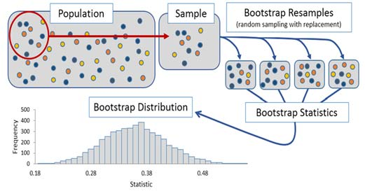
From a theoretical perspective, the ideal scenario for making inferences about a population is to have infinitely many (or a very large number of) samples from that population. If the statistic of interest, for example the mean, is calculated for each sample, what is known as the sampling distribution is obtained. This distribution has two characteristics: its average tends to converge with the true value of the population parameter, and its dispersion allows knowing the expected error when estimating the statistic with a sample of a given size.
In practice, it is usually not possible to access multiple samples. If only one sample is available, and it is representative of the population, values in the sample should appear approximately with the same frequency as in the population. The bootstrapping method (Bradley Efron, 1979)) is based on generating new pseudo-samples, of the same size as the original sample, through repeated sampling with replacement from the available data.
If the original sample is representative of the population, the distribution of the statistic calculated from the pseudo-samples (bootstrapping distribution) approximates the sampling distribution that would be obtained if the population could be accessed to generate new samples.
Thus, bootstrapping is a simulation process through which the sampling distribution of a statistic can be approximated using only an initial sample. However, it is important to highlight what information can and cannot be extracted.
Bootstrapping does not provide a better estimate of the statistic than that obtained with the original sample.
Bootstrapping simulates the sampling process and thereby the variability generated by this process. Thanks to this, it allows estimating the uncertainty that can be expected from a statistic calculated from a sample.
The bootstrapping strategy can be used to solve several problems:
Calculate confidence intervals for a population parameter.
Calculate the statistical significance (p-value) of the difference between populations.
Calculate confidence intervals for the difference between populations.
In each case, the null hypothesis is different and, therefore, the sampling simulation that must be performed. This means that, although similar, the algorithm must be adapted to each use case. The following sections show examples of different applications.
Confidence intervals for a population parameter
Suppose there is a set of $n$ observations $X = \{x_1, x_2, \ldots, x_n\}$ drawn from a distribution (population). The sample mean ($\hat{X}$) is the best approximation to estimate the population mean ($\mu$), but how much uncertainty exists regarding this estimate? That is, how much can the value of $\hat{X}$ be expected to deviate from $\mu$? This question can be answered by calculating confidence intervals (frequentist approach) or with credible intervals (Bayesian approach).
There are several methods to estimate confidence intervals using bootstrapping:
- Normal-based intervals (normal bootstrap intervals)
- Percentile-based intervals (percentile bootstrap intervals)
- Student's t-based intervals (bootstrap Student's t intervals)
- Bias-Corrected and Accelerated Bootstrap Method (BCa)
- Empirical intervals (empirical bootstrap intervals)
This document describes how to calculate percentile-based intervals, empirical intervals, and Bias-Corrected and Accelerated Bootstrap Method (BCa). Although the first two approaches are more intuitive, the statistical community seems to agree that it is most appropriate to use Bias-Corrected and Accelerated Bootstrap Method (BCa). A detailed implementation of this approach can be found in BE/Bi 103 a: Introduction to Data Analysis in the Biological Sciences.
✏️ Note
All of the above also applies to any other statistic (median, trimmed mean...), not just the mean.
Percentile-based intervals
Percentile-based intervals are based on the idea that the simulated distribution resembles the sampling distribution of the statistic, and that its standard deviation approximates the standard error of that distribution. According to this, the confidence interval of the statistic can be estimated using the percentiles of the obtained distribution.
The steps to follow are:
1) Generate $B$ new samples through bootstrapping.
2) Calculate the statistic of interest in each new sample.
3) Calculate the lower and upper quantiles according to the desired interval.
4) Generate the confidence interval as [lower quantile, upper quantile].
For example, the 95% confidence interval obtained from 1000 bootstrapping samples is the interval between the 0.025 quantile and the 0.975 quantile of the obtained distribution.
A sample consisting of 30 observations from a continuous random variable is available. A 95% confidence interval for the mean is to be calculated using the percentile-based bootstrapping method.
The data used in this example were obtained from the book Comparing Groups Randomization and Bootstrap Methods Using R.
# Data processing
# ==============================================================================
import pandas as pd
import numpy as np
from scipy import stats
# Graphics
# ==============================================================================
import matplotlib.pyplot as plt
import seaborn as sns
plt.style.use('ggplot')
# Warnings configuration
# ==============================================================================
import warnings
warnings.filterwarnings('once')
# Miscellaneous
# ==============================================================================
from tqdm.auto import tqdm
# Data
# ==============================================================================
data = np.array([
81.372918, 25.700971, 4.942646, 43.020853, 81.690589, 51.195236,
55.659909, 15.153155, 38.745780, 12.610385, 22.415094, 18.355721,
38.081501, 48.171135, 18.462725, 44.642251, 25.391082, 20.410874,
15.778187, 19.351485, 20.189991, 27.795406, 25.268600, 20.177459,
15.196887, 26.206537, 19.190966, 35.481161, 28.094252, 30.305922
])
# Observed distribution plots
# ==============================================================================
fig, axs = plt.subplots(nrows=1, ncols=2, figsize=(8, 4))
axs[0].hist(data, bins=30, density=True, color='#3182bd', alpha=0.5, label = 'sample_1')
axs[0].plot(data, np.full_like(data, -0.001), '|k', markeredgewidth=1)
axs[0].set_title('Distribution of observed values')
axs[0].set_xlabel('value')
axs[0].set_ylabel('density')
pd.Series(data).plot.kde(ax=axs[1],color='#3182bd')
axs[1].plot(data, np.full_like(data, 0), '|k', markeredgewidth=1)
axs[1].set_title('Estimated density distribution')
axs[1].set_xlabel('value')
axs[1].set_ylabel('density')
fig.tight_layout();

The graphical representation shows evidence that the data is not normally distributed. This implies that the approach based on the central limit theorem to estimate the standard error $SE = \dfrac{sd}{\sqrt{n}}$ may not be accurate with this sample size, and with it, the parametric intervals based on the structure $[\text{estimated parameter} \pm t_\alpha SE]$. An alternative for calculating confidence intervals is to use bootstrapping.
Through bootstrapping, the expected variability in the statistic, in this case the mean, is simulated due solely to random sampling.
def calculate_statistic(x):
'''
Function to calculate the statistic of interest.
Parameters
----------
x : numpy array
sample values.
Returns
-------
statistic: float
Value of the statistic.
'''
statistic = np.mean(x)
return statistic
def bootstrapping(x, fun_statistic, n_iterations=9999, random_state=98752):
'''
Function to calculate the value of the statistic in multiple samples generated
through repeated sampling with replacement (bootstrapping).
Parameters
----------
x : numpy array
Sample values.
fun_statistic : function
Function that receives a sample as argument and returns the value
of the statistic.
n_iterations : int, default `9999`
Number of iterations.
random_state : int, default `98752`
Seed for random number generator.
Returns
-------
distributions: numpy array
Value of the statistic in each bootstrap sample.
'''
rng = np.random.default_rng(random_state)
n = len(x)
boot_dist = np.full(shape=n_iterations, fill_value=np.nan)
for i in tqdm(range(n_iterations)):
resample = rng.choice(x, size=n, replace=True)
boot_dist[i] = fun_statistic(resample)
return boot_dist
# Bootstrapping process
# ==============================================================================
boot_dist = bootstrapping(
x = data,
fun_statistic = calculate_statistic,
n_iterations = 9999,
random_state = 98752
)
0%| | 0/9999 [00:00<?, ?it/s]
# Bootstrap distribution
# ==============================================================================
fig, ax = plt.subplots(ncols=1, nrows=1, figsize=(7,3))
ax.hist(boot_dist, bins=30, density=True, color='#3182bd', alpha=0.5)
ax.set_title('Bootstrap distribution')
ax.set_xlabel('mean')
ax.set_ylabel('density');

The dispersion of the distribution obtained by bootstrapping is an approximation of the expected standard error due to the sampling process. For this reason, its percentiles can be used to calculate confidence intervals.
# Confidence interval (CI) based on bootstrap distribution percentiles
# ==============================================================================
# A 95% CI should span from the 0.025 to the 0.975 quantile
quantiles = np.quantile(a = boot_dist, q = [0.025, 0.975])
print('------------------------------')
print('Percentile-based interval')
print('------------------------------')
print(quantiles)
------------------------------ Percentile-based interval ------------------------------ [25.00638973 37.77271182]
# 95% confidence interval plot
# ==============================================================================
fig, ax = plt.subplots(ncols=1, nrows=1, figsize=(7,3))
ax.hist(boot_dist, bins=30, density=True, color='#3182bd', alpha=0.5)
ax.axvline(x=data.mean(), color='red', label='observed mean')
ax.axvline(x=quantiles[0], color='black', linestyle='--', label='95% CI')
ax.axvline(x=quantiles[1], color='black', linestyle='--')
ax.hlines(y=0.001, xmin=quantiles[0], xmax=quantiles[1], color='black')
ax.set_title('Percentile-based bootstrap interval')
ax.set_xlabel('mean')
ax.set_ylabel('density')
ax.legend();

Empirical intervals
The percentile-based approach estimates the expected difference between the sample mean $\hat{X}$ and the population mean $\mu$ from the dispersion of the distribution obtained through bootstrapping. Instead of this, the empirical approach tries to directly estimate the expected difference between the sample mean $\hat{X}$ and the population mean $\mu$ from the differences between the sample mean $\hat{X}$ and the means of each bootstrapping iteration $\hat{X}^{b_i}$.
Starting from the following elements:
$X$: sample consisting of $n$ observations.
$$X = \{x_1, x_2, \ldots, x_n\}$$$\mu$: population mean, whose value is unknown and about which inference is to be made.
$\hat{X}$: sample mean, mean calculated with the observed values.
$\hat{X}^b$: mean of a sample generated by bootstrapping.
$V$: expected difference of $\hat{X}$ with respect to $\mu$.
$$V = \hat{X} - \mu$$$\hat{V}^b$: difference of $\hat{X}^b$ with respect to $\hat{X}$.
$$\hat{V}^b = \hat{X}^b - \hat{X}$$
According to the law of large numbers, the distribution of $\hat{X}$ is centered on $\mu$. Hence, the best available estimate of the population mean is the sample mean. Similarly, the distribution of $\hat{X}^b$ obtained by bootstrapping from $X$ is centered on $\hat{X}$.
On the other hand, the distribution of $V = \hat{X} - \mu$ represents the variation of the sample mean with respect to the population mean. This is what is desired to obtain the confidence interval. Since $\mu$ is unknown, there is no way to directly calculate the distribution of $V$. However, it can be approximated from the differences between the means of the bootstrap samples and the sample mean.
$$\hat{V}^b = \hat{X}^b - \hat{X}$$Once the distribution of $\hat{V}^b$ is obtained, the confidence interval for $\mu$ can be obtained:
$$\text{95\% confidence interval} = [\hat{X} - \hat{V}^b_{0.975},\ \hat{X} - \hat{V}^b_{0.025}]$$where $\hat{V}^b_{0.025}$ and $\hat{V}^b_{0.975}$ are the respective quantiles of the distribution of $\hat{V}^b$ obtained by bootstrapping.
Algorithm
The steps to follow to calculate intervals using the empirical approach are:
1) Calculate the sample mean $\hat{X}$
2) Obtain $B$ bootstrapping samples through repeated sampling.
3) For each bootstrapping sample:
- Calculate the mean $\hat{X}^b$
- Calculate the difference $\hat{V}^b=\hat{X}^b-\hat{X}$
4) Calculate the quantiles corresponding to the interval of interest from the values $\hat{V}^b$
5) Calculate the confidence interval as $\hat{X} - \text{quantiles}$
✏️ Note
Both the percentile and empirical approaches use quantiles, but there is an important difference. In the first, they are calculated directly on the distribution of the statistic, while in the empirical approach, they are calculated on the distribution of variation.
Suppose again the case shown in the previous example. A sample consisting of 30 observations from a continuous random variable is available. A 95% confidence interval for the mean is to be calculated, but this time, using the empirical bootstrapping method.
Unlike the other approaches, in empirical bootstrapping, the simulated distribution is not that of the statistic of interest (the mean in this case), but that of the deviations between the statistic calculated with the original sample and the statistic obtained in each bootstrap sample.
def calculate_statistic(x):
'''
Function to calculate the statistic of interest.
Parameters
----------
x : numpy array
sample values.
Returns
-------
statistic: float
value of the statistic.
'''
statistic = np.mean(x)
return(statistic)
def bootstrapping_empirical(x, fun_statistic, n_iterations=9999, random_state=98752):
'''
Function to calculate the difference between the value of the statistic in the
original sample and the value of the statistic in multiple samples generated
by sampling with replacement.
Parameters
----------
x : numpy array
Sample values.
fun_statistic : function
Function that receives a sample as argument and returns the value
of the statistic.
n_iterations : int
Number of iterations (default `9999`).
Returns
-------
Distributions: numpy array
Value of the statistic difference in each bootstrap sample.
'''
rng = np.random.default_rng(random_state)
n = len(x)
sample_statistic = fun_statistic(x)
boot_dist = np.full(shape=n_iterations, fill_value=np.nan)
for i in tqdm(range(n_iterations)):
resample = rng.choice(x, size=n, replace=True)
boot_dist[i] = fun_statistic(resample) - sample_statistic
return boot_dist
# Bootstrapping process
# ==============================================================================
boot_dist = bootstrapping_empirical(
x = data,
fun_statistic = calculate_statistic,
n_iterations = 9999,
random_state = 98752
)
0%| | 0/9999 [00:00<?, ?it/s]
# Bootstrap distribution
# ==============================================================================
fig, ax = plt.subplots(ncols=1, nrows=1, figsize=(7,3))
ax.hist(boot_dist, bins=30, density=True, color='#3182bd', alpha=0.5)
ax.set_title('Bootstrap distribution')
ax.set_xlabel(r'$\hat{X}^{b} - \hat{X}$')
ax.set_ylabel('density');

The distribution obtained by bootstrapping is an approximation of the difference that can be expected between the value of the statistic calculated with the available sample data and the true value of the population parameter. In this specific example, it represents the difference that can be expected between the sample mean and the population mean value.
# Confidence interval (CI) based on empirical bootstrapping.
# ==============================================================================
# A 95% CI should span from the 0.025 to the 0.975 quantile
quantiles = np.quantile(a = boot_dist, q = [0.025, 0.975])
sample_statistic = calculate_statistic(data)
print('------------------')
print('Empirical interval')
print('------------------')
interval = [float(sample_statistic - quantiles[1]) , float(sample_statistic - quantiles[0])]
print(interval)
------------------ Empirical interval ------------------ [24.164600045000007, 36.93092213666667]
Bias-Corrected and Accelerated Bootstrap Method (BCa)
The code shown in the previous examples, while offering a clear view of the bootstrapping process, is not computationally efficient. Scipy offers a function called bootstrap that implements bootstrapping methods in an optimized way. In addition to being more efficient, this function implements the Bias-Corrected and Accelerated Bootstrap Method (BCa), which is considered the most appropriate method for calculating confidence intervals using bootstrapping.
# Bootstrapping process using scipy.stats.bootstrap
# ==============================================================================
bootstrapped_result = stats.bootstrap(
data = (data,),
statistic = calculate_statistic,
n_resamples = 9999,
method = 'BCa',
random_state = 98752
)
interval_bca = list(bootstrapped_result.confidence_interval)
print('------------------')
print('BCa interval')
print('------------------')
print(interval_bca)
------------------ BCa interval ------------------ [np.float64(25.518666166207176), np.float64(39.119061531884)]
# 95% confidence interval plot
# ==============================================================================
fig, ax = plt.subplots(ncols=1, nrows=1, figsize=(7,3))
ax.hist(bootstrapped_result.bootstrap_distribution, bins=30, density=True, color='#3182bd', alpha=0.5)
ax.axvline(x=data.mean(), color='red', label='observed mean')
ax.axvline(x=interval_bca[0], color='black', linestyle='--', label='95% CI')
ax.axvline(x=interval_bca[1], color='black', linestyle='--')
ax.hlines(y=0.001, xmin=interval_bca[0], xmax=interval_bca[1], color='black')
ax.set_title('Percentile-based bootstrap interval')
ax.set_xlabel('mean')
ax.set_ylabel('density')
ax.legend();

Intervals with parametric methods
The obtained intervals are compared with the intervals estimated if a parametric model based on a Student's t-distribution is used.
# Intervals with parametric methods (Student's t)
# ==============================================================================
interval = stats.t.interval(
0.95,
df=len(data)-1,
loc=np.mean(data),
scale=stats.sem(data)
)
print('----------------------')
print('Student\'s t interval')
print('--------------------')
print(interval)
---------------------- Student's t interval -------------------- (np.float64(24.113169102822646), np.float64(37.82414276384402))
Calculating p-value
Bootstrapping as a significance test for the difference between groups is used when studying whether the difference between two populations is significant (p-value).
While this use resembles that of permutation tests, it is not equivalent.
Permutation tests contrast the null hypothesis that samples belong to the same population (distribution) through the study of differences due to random group assignment.
With the bootstrapping method, the hypothesis that both samples come from the same population (distribution) is also tested, but it is done through the study of differences due to random sampling. It applies to scenarios where there has been no random group assignment, but samples have been obtained from already separated groups.
The steps to follow to apply bootstrapping to this type of test are:
1) Mix the observations from both samples (pool).
2) Use sampling with replacement on this pool to generate a new pseudo-sample of the same size.
3) Separate the observations from the pseudo-sample into two groups of equal size to the original ones.
4) Calculate the difference of the statistic between both.
5) Repeat steps 2, 3, and 4 multiple times, thus generating the distribution of expected differences due to random sampling.
6) Calculate the two-tailed p-value as the proportion of pseudo-samples in which the absolute value of the calculated difference is greater than or equal to the absolute value of the observed difference.
Example
A study aims to determine whether there is a difference between the average academic achievements of students from two different countries. To do this, a random sample of students from both origins who arrived in the country between 2005 and 2006 is obtained.
Since this is a sampling design, in which a random sample with individuals from each group has been obtained, the bootstrapping method is appropriate.
The data used in this example were obtained from the book Comparing Groups Randomization and Bootstrap Methods Using R.
# Data
# ==============================================================================
url = 'https://raw.githubusercontent.com/JoaquinAmatRodrigo/Estadistica-con-R/' \
+ 'master/datos/LatinoEd.csv'
data = pd.read_csv(url)
data = data[['Achieve', 'Mex']]
data = data.rename(columns={'Achieve': 'score', 'Mex': 'nationality'})
data['nationality'] = np.where(data['nationality'] == 0, 'country_1', 'country_2')
data.head(4)
| score | nationality | |
|---|---|---|
| 0 | 59.2 | country_2 |
| 1 | 63.7 | country_2 |
| 2 | 62.4 | country_2 |
| 3 | 46.8 | country_2 |
The average academic performance is 5.92 points lower in students from country 1.
# Descriptive statistics by group
# ==============================================================================
data.groupby(by='nationality').describe()
| score | ||||||||
|---|---|---|---|---|---|---|---|---|
| count | mean | std | min | 25% | 50% | 75% | max | |
| nationality | ||||||||
| country_1 | 34.0 | 64.514706 | 13.031410 | 29.3 | 58.675 | 66.65 | 70.20 | 87.8 |
| country_2 | 116.0 | 58.593103 | 15.626876 | 21.5 | 50.100 | 60.80 | 68.45 | 96.2 |
# Observed mean difference between groups
# ==============================================================================
observed_diff = (
data.loc[data['nationality'] == 'country_1', 'score'].mean()
- data.loc[data['nationality'] == 'country_2', 'score'].mean()
)
print(f"Observed mean difference: {observed_diff}")
Observed mean difference: 5.921602434077073
# Observed distribution plots
# ==============================================================================
fig, axs = plt.subplots(nrows=1, ncols=2, figsize=(8, 3.5))
# Create color mapping for each nationality
nationalities = data['nationality'].unique()
colors = plt.cm.tab10.colors
color_map = {nat: colors[i] for i, nat in enumerate(nationalities)}
sns.violinplot(
x = data['score'],
y = data['nationality'],
color = ".8",
ax = axs[0]
)
sns.stripplot(
x = data['score'],
y = data['nationality'],
hue = 'nationality',
data = data,
size = 4,
jitter = 0.1,
palette = 'tab10',
legend = False,
ax = axs[0]
)
axs[0].set_ylabel('nationality')
axs[0].set_xlabel('score');
for nationality in nationalities:
data_temp = data.loc[data['nationality'] == nationality, 'score']
data_temp.plot.kde(ax=axs[1], label=nationality, color=color_map[nationality])
axs[1].plot(data_temp, np.full_like(data_temp, 0), '|k', markeredgewidth=1)
axs[1].set_xlabel('score');
axs[1].legend()
fig.suptitle('Comparison of academic performance by nationality', fontsize=12)
fig.tight_layout();

Bootstrapping distribution
The objective of the study is to determine if the observed difference of 5.9 units is within what could be expected solely due to random sampling, if there were no real difference between the populations:
$$H_0: \text{all observations come from the same population}$$If a new sample of students were obtained, the average difference between groups would be slightly different, even if there were no real difference between nationalities. Therefore, answering this problem involves determining how much difference is expected simply by repeating the sampling.
Through bootstrapping, new pseudo-samples of individuals are generated using the two original samples (country 1 and country 2) combined. With each of the pseudo-samples, two groups are generated with sizes equal to those of the original sample groups (34, 116) and the difference of the statistic is calculated, in this case the mean. The process is very similar to that used in permutation tests. The difference lies in the fact that, in permutation tests, the observations from the original sample are always used, ordered differently in each iteration. In this case, in each iteration and before the group assignment, a new pseudo-sample is generated that has the same size as the original sample but formed by different observations.
def calculate_statistic(x):
'''
Function to calculate the statistic of interest.
Parameters
----------
x : numpy array
sample values.
Returns
-------
statistic: float
value of the statistic.
'''
statistic = np.mean(x)
return(statistic)
def bootstrapping_2_groups(x1, x2, fun_statistic, n_iterations=9999, random_state=98752):
'''
Function to calculate the difference of a statistic between two groups in
multiple samples generated through repeated sampling with replacement
(bootstrapping). This function is designed for hypothesis testing (p-value
calculation) and pools both samples before resampling to simulate the null
hypothesis that both groups come from the same population.
Parameters
----------
x1 : numpy array
values of the sample from group 1.
x2 : numpy array
values of the sample from group 2.
fun_statistic : function
function that receives a sample as argument and returns the value
of the statistic.
n_iterations : int
number of iterations (default `9999`).
random_state : int
seed for random number generator (default `98752`).
Returns
-------
distributions: numpy array
difference between both groups in each bootstrap sample.
'''
rng = np.random.default_rng(random_state)
n1 = len(x1)
n2 = len(x2)
pool = np.hstack((x1, x2))
boot_dist = np.full(shape=n_iterations, fill_value=np.nan)
for i in tqdm(range(n_iterations)):
# Create a new sample
resample = rng.choice(pool, size=n1+n2, replace=True)
# Split observations into two groups and calculate the statistic
statistic_1 = fun_statistic(resample[:n1])
statistic_2 = fun_statistic(resample[n1:])
# Difference between statistics
boot_dist[i] = statistic_1 - statistic_2
return boot_dist
# Bootstrapping process
# ==============================================================================
boot_dist = bootstrapping_2_groups(
x1 = data.loc[data['nationality'] == 'country_1', 'score'],
x2 = data.loc[data['nationality'] == 'country_2', 'score'],
fun_statistic = calculate_statistic,
n_iterations = 9999
)
0%| | 0/9999 [00:00<?, ?it/s]
The simulated data form what is known as the bootstrapping distribution and represents the expected variation in the difference of means solely due to random sampling, if both samples come from the same population.
# Bootstrap distribution
# ==============================================================================
observed_diff = data.score[data.nationality == 'country_1'].mean() \
- data.score[data.nationality == 'country_2'].mean()
fig, ax = plt.subplots(ncols=1, nrows=1, figsize=(7, 3))
ax.hist(boot_dist, bins=30, density=True, color='#3182bd', alpha=0.5)
ax.axvline(x=observed_diff, color='red', label='observed difference')
ax.axvline(x=-observed_diff, color='red')
ax.set_title('Bootstrap distribution')
ax.set_xlabel('mean difference')
ax.set_ylabel('density')
ax.legend();

pd.Series(boot_dist).describe()
count 9999.000000 mean 0.024777 std 3.030201 min -11.879209 25% -2.014782 50% 0.051166 75% 2.091278 max 12.583316 dtype: float64
As expected, the difference between the mean of the groups, considering that all come from the same population, is centered on zero.
p-value
Finally, the probability (p-value) of obtaining differences equal to or more extreme than the observed one (red vertical lines) is calculated.
# Empirical p-value with and without correction
# ==============================================================================
p_value = (sum(np.abs(boot_dist) >= np.abs(observed_diff)))/len(boot_dist)
p_value_correc = (sum(np.abs(boot_dist) >= np.abs(observed_diff)) + 1)/(len(boot_dist) + 1)
print(f"p-value without correction: {p_value}")
print(f"p-value with correction: {p_value_correc}")
p-value without correction: 0.050505050505050504 p-value with correction: 0.0506
Conclusion
A nonparametric bootstrapping test was used to determine whether there is a difference in the average academic achievements between students from two different nationalities. The data was obtained through random sampling, thus ensuring data independence. The p-value was calculated using 9999 Monte Carlo simulations, employing the continuity correction suggested by Davison and Hinkley (1997). The obtained result (p-value) is moderate evidence against the null hypothesis that there is no difference between populations.
⚠️ Important
scipy.stats.bootstrap is not suitable for calculating p-values in group comparison hypothesis tests. The function is designed to calculate confidence intervals, not to perform hypothesis testing. The fundamental difference is that:
- For confidence intervals: each group is resampled separately, maintaining the structure of observed differences.
- For hypothesis tests (p-value): the null hypothesis $H_0$ (both groups come from the same population) must be implemented by resampling once from the combined pool and then separating into groups.
Even if pooled data is passed to scipy.stats.bootstrap, the function creates independent resamples for each data argument, which does not correctly implement the null hypothesis. What is needed is:
- Create a single resample from the combined pool
- Split that resample into two groups of sizes n₁ and n₂
- Calculate the difference between both
Confidence intervals for the difference between populations
For this use of bootstrapping, the null hypothesis is that the observations come from two different populations. Repeated sampling is used with the observations from each sample (without mixing them) to generate two new independent pseudo-samples and the difference of the statistic is calculated. This process is repeated multiple times, thus generating the distribution that would be obtained if two samples were obtained each time, each from its respective population, and the difference were calculated.
Hypothesis tests that contrast the difference between two populations generate a p-value based on the null hypothesis that there is no difference in the statistic (mean, median...) between the populations. For this reason, when bootstrapping is used as a hypothesis test, the observations are all mixed together and, subsequently, the pseudo-samples are generated. When the purpose of the study is to generate confidence intervals for the true difference of a statistic between two populations, the null hypothesis considers that the samples do come from two different populations, each with a different value for the studied statistic. To simulate this null hypothesis, the pseudo-samples obtained by sampling with replacement must be generated separately for each group. This is the difference between the use of bootstrapping to calculate p-values and to calculate confidence intervals of differences.
The bootstrapping algorithm to calculate confidence intervals for the difference between two populations is:
1) Generate a new pseudo-sample from group $A$ of the same size as the original sample $n_A$ using only the observations belonging to that group.
2) Generate a new pseudo-sample from group B of the same size as the original sample $n_B$ using only the observations belonging to that group.
3) Calculate the difference of the statistic between the two new pseudo-samples.
4) Repeat steps 1, 2, and 3 multiple times, storing the difference calculated in each iteration. The distribution of the generated values represents the difference of the statistic if both samples come from two different populations. This distribution tends to be centered on the true value of the difference between both populations.
5) From the obtained distribution, generate a confidence interval for the population parameter. The same considerations explained for confidence intervals in a single population also apply to the difference between populations.
Example
There is a dataset with information about the time a telecommunications company takes to repair problems for two consumer groups (CLEC and ILEC). The goal is to know what the difference is in the mean repair times of both groups using a 95% confidence interval.
The data used in this example was obtained from the R package resample.
# Data
# ==============================================================================
url = (
'https://raw.githubusercontent.com/JoaquinAmatRodrigo/Estadistica-machine-learning-python/'
'master/data/verizon.csv'
)
data = pd.read_csv(url)
data.head(3)
| Time | Group | |
|---|---|---|
| 0 | 17.5 | ILEC |
| 1 | 2.4 | ILEC |
| 2 | 0.0 | ILEC |
# Descriptive statistics by group
# ==============================================================================
data.groupby(by='Group').describe()
| Time | ||||||||
|---|---|---|---|---|---|---|---|---|
| count | mean | std | min | 25% | 50% | 75% | max | |
| Group | ||||||||
| CLEC | 23.0 | 16.509130 | 19.503576 | 0.0 | 5.425 | 14.33 | 20.715 | 96.32 |
| ILEC | 1664.0 | 8.411611 | 14.690039 | 0.0 | 0.730 | 3.59 | 7.080 | 191.60 |
# Observed mean difference between groups
# ==============================================================================
observed_diff = (data.Time[data.Group == 'CLEC'].mean()
- data.Time[data.Group == 'ILEC'].mean())
print(f"Observed mean difference: {observed_diff}")
Observed mean difference: 8.097519857859533
# Observed distribution plots
# ==============================================================================
fig, axs = plt.subplots(nrows=1, ncols=2, figsize=(8, 3.5))
# Create color mapping for each group
groups = data['Group'].unique()
colors = plt.cm.tab10.colors
color_map = {group: colors[i] for i, group in enumerate(groups)}
sns.violinplot(
x = data['Time'],
y = data['Group'],
color = ".8",
ax = axs[0]
)
sns.stripplot(
x = data['Time'],
y = data['Group'],
hue = 'Group',
data = data,
size = 4,
jitter = 0.1,
palette = 'tab10',
legend = False,
ax = axs[0]
)
axs[0].set_ylabel('group')
axs[0].set_xlabel('time');
for group in data.Group.unique():
data_temp = data.loc[data['Group'] == group, 'Time']
data_temp.plot.kde(ax=axs[1], label=group, color=color_map[group])
axs[1].plot(data_temp, np.full_like(data_temp, 0), '|k', markeredgewidth=1)
axs[1].set_xlim(0)
axs[1].set_xlabel('time');
axs[1].legend()
fig.suptitle('Comparison of response times by group', fontsize=12)
fig.tight_layout();

The graphical representation shows a marked asymmetry of the data. Additionally, the size of one of the groups is only 23 observations. Parametric methods based on the central limit theorem, such as the t-test, may not be appropriate in this scenario.
Bootstrap distribution
Through bootstrapping, new pseudo-samples are obtained separately from each of the initial samples maintaining the original size and the difference is calculated.
def calculate_statistic(x):
'''
Function to calculate the statistic of interest.
Parameters
----------
x : numpy array
sample values.
Returns
-------
statistic: float
value of the statistic.
'''
statistic = np.mean(x)
return(statistic)
def bootstrapping_2_groups(x1, x2, fun_statistic, n_iterations=9999, random_state=98752):
'''
Function to calculate the difference of a statistic between two groups in
multiple samples generated through repeated sampling with replacement
(bootstrapping) separately for each group. This function is designed for
calculating confidence intervals for the difference between populations,
and samples from each group independently to preserve their distinct
distributions.
Parameters
----------
x1 : numpy array
Values of the sample from group 1.
x2 : numpy array
Values of the sample from group 2.
fun_statistic : function
Function that receives a sample as argument and returns the value
of the statistic.
n_iterations : int
number of iterations (default `9999`).
random_state: int
seed for random number generator (default `98752`).
Returns
-------
distributions: numpy array
difference between both groups in each bootstrap sample.
'''
rng = np.random.default_rng(random_state)
n1 = len(x1)
n2 = len(x2)
boot_dist = np.full(shape=n_iterations, fill_value=np.nan)
for i in tqdm(range(n_iterations)):
# Create a new sample from each group
resample_1 = rng.choice(x1, size=n1, replace=True)
resample_2 = rng.choice(x2, size=n2, replace=True)
# Calculate the statistic for each group
statistic_1 = fun_statistic(resample_1)
statistic_2 = fun_statistic(resample_2)
# Difference between statistics
boot_dist[i] = statistic_1 - statistic_2
return boot_dist
boot_dist = bootstrapping_2_groups(
x1 = data.loc[data['Group'] == 'CLEC', 'Time'],
x2 = data.loc[data['Group'] == 'ILEC', 'Time'],
fun_statistic = calculate_statistic,
n_iterations = 9999
)
0%| | 0/9999 [00:00<?, ?it/s]
The simulated data forms what is known as the bootstrapping distribution and represents the expected variation in the difference of means solely due to random sampling, assuming that both samples come from two different populations.
# CI based on bootstrap distribution percentiles
# ==============================================================================
# A 95% CI should span from the 0.025 to the 0.975 quantile
quantiles = np.quantile(a = boot_dist, q = [0.025, 0.975])
print('------------------------------')
print('Percentile-based interval')
print('------------------------------')
print(quantiles)
------------------------------ Percentile-based interval ------------------------------ [ 1.72798217 17.44282553]
# 95% confidence interval plot
# ==============================================================================
fig, ax = plt.subplots(ncols=1, nrows=1, figsize=(7,3))
ax.hist(boot_dist, bins=30, density=True, color='#3182bd', alpha=0.5)
ax.axvline(x=observed_diff, color='red', label='observed difference')
ax.axvline(x=quantiles[0], color='black', linestyle='--', label='95% CI')
ax.axvline(x=quantiles[1], color='black', linestyle='--')
ax.hlines(y=0.001, xmin=quantiles[0], xmax=quantiles[1], color='black')
ax.set_title('Percentile-based bootstrap interval')
ax.set_xlabel('mean')
ax.set_ylabel('density')
ax.legend();

Conclusion
There is evidence to affirm that the average repair time between the two groups is different. The 95% confidence interval for the difference in means obtained by bootstrapping indicates that, on average, CLEC group repairs take 1.7 to 17 hours longer.
# CI based on BCa with scipy.stats.bootstrap
# ==============================================================================
def calculate_statistic_diff(x, y, axis=0):
'''
Function to calculate the difference of the statistic of interest between two groups.
Parameters
----------
x : numpy array
values of the sample from group 1.
y : numpy array
values of the sample from group 2.
axis : int, optional
axis over which to operate (required by scipy.stats.bootstrap).
Returns
-------
statistic: float
value of the statistic.
'''
statistic = np.mean(x, axis=axis) - np.mean(y, axis=axis)
return(statistic)
bootstrapped_result = stats.bootstrap(
data = (
data.loc[data['Group'] == 'CLEC', 'Time'],
data.loc[data['Group'] == 'ILEC', 'Time']
),
statistic = calculate_statistic_diff,
n_resamples = 9999,
method = 'BCa',
random_state = 98752
)
interval_bca = list(bootstrapped_result.confidence_interval)
print('------------------')
print('BCa interval')
print('------------------')
print(interval_bca)
------------------ BCa interval ------------------ [np.float64(2.842646968873678), np.float64(21.22624762011161)]
Comparison of bootstrapping and permutations
Both permutation tests and bootstrapping tests can be used to study differences between groups. There is a very extensive list of references debating which of the two methods is most appropriate. In general, they all agree that the most appropriate method depends on the objective of the inference, and in turn, the possible objectives are constrained by the study design followed. The following table contains the different types of designs that can be used to compare two groups and the type of inference (conclusions) that can be made in each one:
| Random sampling | Random group assignment | Inference objective | Allows determining causality |
|---|---|---|---|
| Yes | No | Population | No |
| No | Yes | Sample | Yes |
| Yes | Yes | Population and Sample | Yes |
The main difference between both methods appears when they are used to calculate p-values. Significance tests (calculation of p-value) are based on the null hypothesis that all observations come from the same population. The objective of the test is to determine whether the observed difference between groups is due to a particular factor (treatment) or only to the expected variability by the nature of a random process.
When randomness is due to the assignment of subjects to different groups, permutation tests are used. The structure of an experiment that can be analyzed using permutation tests is:
Selection of study subjects.
Random assignment to different groups
Application of "treatment" and comparison of results.
Permutation tests answer the question: How much variability is expected in a given statistic solely due to the randomness of assignments, if all subjects really come from the same population? When comparing the mean between two groups, the previous question is equivalent to: What difference between means can be expected depending on how subjects are distributed in the two groups, if all come from the same population? (Even if they are all from the same population, since they will not be exactly identical, there will be small differences depending on how they are grouped).
Bootstrapping as a significance test is used when randomness is due to the sample obtaining process and not to group assignment. It answers the question: How much variability is expected in a given statistic solely due to random sampling, if all subjects really come from the same population? Due to the small differences between individuals in a population, if two random samples are drawn from it and compared, they will not be exactly equal, and this difference will be different for each pair of random samples drawn. The structure of an experiment that can be analyzed using bootstrapping is:
Two random samples are obtained from two populations.
They are compared.
In conclusion, although both tests can be used to calculate p-values, their applications do not overlap. Permutation and randomization tests are used for experimental designs, while bootstrapping is used for sampling designs.
It is important to keep in mind that none of these methods is free from the problems that having small samples implies.
Session information
import session_info
session_info.show(html=False)
----- matplotlib 3.10.8 numpy 2.2.6 pandas 2.3.3 scipy 1.15.3 seaborn 0.13.2 session_info v1.0.1 tqdm 4.67.1 ----- IPython 9.8.0 jupyter_client 8.7.0 jupyter_core 5.9.1 ----- Python 3.13.11 | packaged by Anaconda, Inc. | (main, Dec 10 2025, 21:28:48) [GCC 14.3.0] Linux-6.14.0-37-generic-x86_64-with-glibc2.39 ----- Session information updated at 2025-12-27 01:50
Bibliography
Comparing groups Randomization and Bootstrap Methods using R. Andrew S.Zieffler
Bootstrap Methods and Permutation Test by Tim Hestemberg
Introduction to Statistical Learning, Gareth James, Daniela Witten, Trevor Hastie and Robert Tibshirani
Points of Significance Sampling distributions and the bootstrap by Anthony Kulesa, Martin Krzywinski, Paul Blainey & Naomi Altman
Citation instructions
How to cite this document?
If you use this document or any part of it, we would appreciate if you cite it. Thank you very much!
Bootstrapping for confidence intervals and hypothesis testing by Joaquín Amat Rodrigo, available under an Attribution-NonCommercial-ShareAlike 4.0 International (CC BY-NC-SA 4.0 DEED) license at https://www.cienciadedatos.net/documentos/pystats04-bootstrapping-python
Did you like the article? Your help is important
Your contribution will help me continue generating free educational content. Thank you very much! 😊


This document created by Joaquín Amat Rodrigo is licensed under Attribution-NonCommercial-ShareAlike 4.0 International.
Permissions:
-
Share: copy and redistribute the material in any medium or format.
-
Adapt: remix, transform and build upon the material.
Under the following terms:
-
Attribution: You must give appropriate credit, provide a link to the license, and indicate if changes were made. You may do so in any reasonable manner, but not in any way that suggests the licensor endorses you or your use.
-
Non-Commercial: You may not use the material for commercial purposes.
-
Share-Alike: If you remix, transform, or build upon the material, you must distribute your contributions under the same license as the original.