More about forecasting in cienciadedatos.net
- ARIMA and SARIMAX models with python
- Time series forecasting with machine learning
- Forecasting time series with gradient boosting: XGBoost, LightGBM and CatBoost
- Forecasting time series with XGBoost
- Global Forecasting Models: Multi-series forecasting
- Global Forecasting Models: Comparative Analysis of Single and Multi-Series Forecasting Modeling
- Probabilistic forecasting
- Forecasting with deep learning
- Forecasting energy demand with machine learning
- Forecasting web traffic with machine learning
- Intermittent demand forecasting
- Modelling time series trend with tree-based models
- Bitcoin price prediction with Python
- Stacking ensemble of machine learning models to improve forecasting
- Interpretable forecasting models
- Mitigating the Impact of Covid on forecasting Models
- Forecasting time series with missing values

Introduction
When trying to predict future values, most forecasting models try to predict what will be the most likely value. This is called point-forecasting. Although knowing the expected value of a time series in advance is useful in almost any business case, this type of prediction does not provide any information about the confidence of the model or the uncertainty of the prediction.
Probabilistic forecasting, as opposed to point-forecasting, is a family of techniques that allow the prediction of the expected distribution of the outcome rather than a single future value. This type of forecasting provides much richer information because it allows the creation of prediction intervals, the range of likely values where the true value may fall. More formally, a prediction interval defines the interval within which the true value of the response variable is expected to be found with a given probability.
Skforecast implements several methods for probabilistic forecasting:
- Bootstrapped residuals: Bootstrapping is a statistical technique that allows for estimating the distribution of a statistic by resampling the data with replacement. In the context of forecasting, bootstrapping the residuals of a model allows for estimating the distribution of the errors, which can be used to create prediction intervals.
Conformal prediction: Conformal prediction is a framework for constructing prediction intervals that are guaranteed to contain the true value with a specified probability (coverage probability). It works by combining the predictions of a point-forecasting model with its past residuals—differences between previous predictions and actual values. These residuals help estimate the uncertainty in the forecast and determine the width of the prediction interval that is then added to the point forecast. Skforecast implements Split Conformal Prediction (SCP).
Conformal methods can also calibrate prediction intervals generated by other techniques, such as quantile regression or bootstrapped residuals. In this case, the conformal method adjusts the prediction intervals to ensure that they remain valid with respect to the coverage probability.
- Quantile regression: Quantile regression is a technique for estimating the conditional quantiles of a response variable. By combining the predictions of two quantile regressors, an interval can be constructed, with each model estimating one of the bounds of the interval. For example, models trained on $Q = 0.1$ and $Q = 0.9$ produce an 80% prediction interval ($90\% - 10\% = 80\%$).
⚠️ Warning
As Rob J Hyndman explains in his blog, in real-world problems, almost all prediction intervals are too narrow. For example, nominal 95% intervals may only provide coverage between 71% and 87%. This is a well-known phenomenon and arises because they do not account for all sources of uncertainty. With forecasting models, there are at least four sources of uncertainty: the random error term, the parameter estimates, the choice of model for the historical data, and the continuation of the historical data generating process into the future. When producing prediction intervals for time series models, generally only the first of these sources is taken into account. Therefore, it is advisable to use test data to validate the empirical coverage of the interval and not only rely on the expected one.
💡 Tip
This is the first in a series of documents on probabilistic forecasting.
Bootstrapped Residuals
Forecasting intervals with bootstrapped residuals is a method used to estimate the uncertainty in predictions by resampling past prediction errors (residuals). The goal is to generate prediction intervals that capture the variability in the forecast, giving a range of possible future values instead of just a single point estimate.
The error of a one-step-ahead forecast is defined as the difference between the actual value and the predicted value ($e_t = y_t - \hat{y}_{t|t-1}$). By assuming that future errors will be similar to past errors, it is possible to simulate different predictions by taking samples from the collection of errors previously seen in the past (i.e., the residuals) and adding them to the predictions.
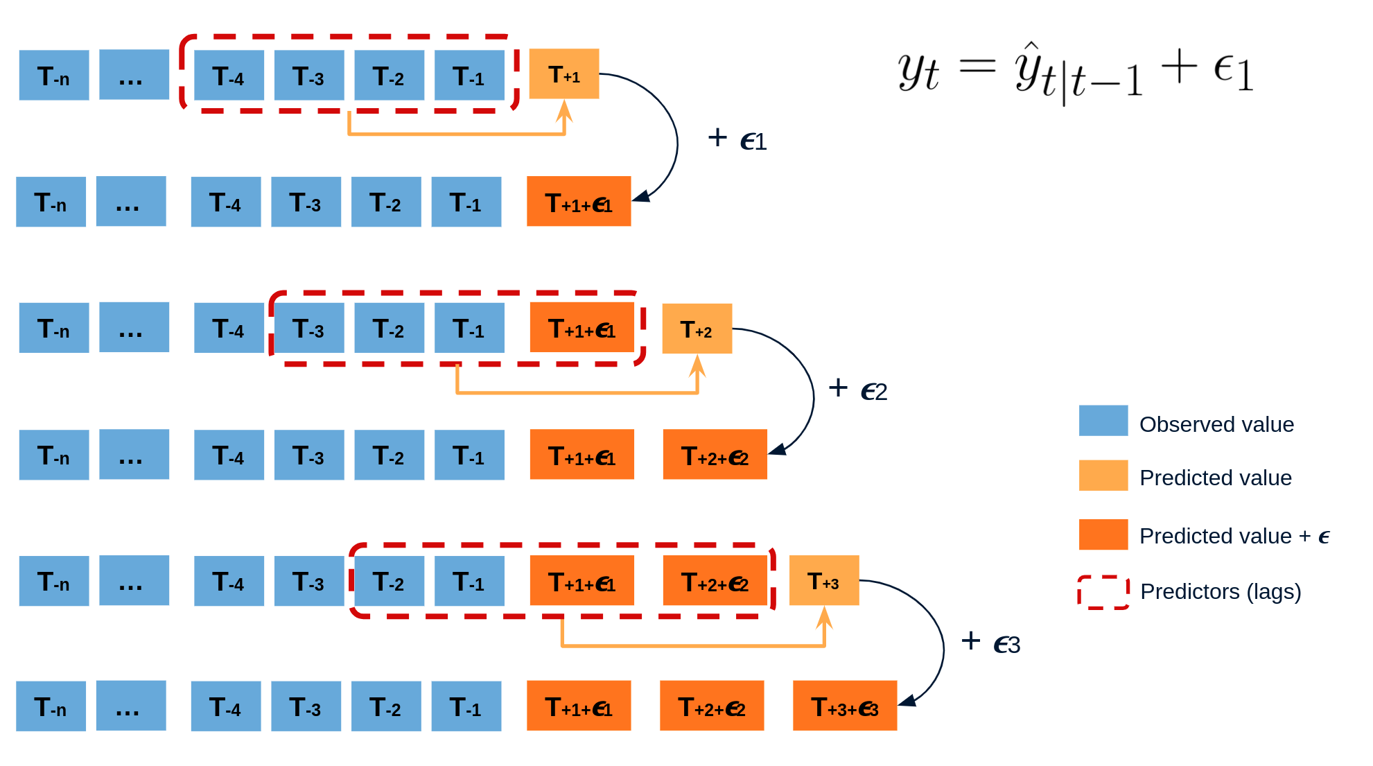
Diagram bootstrapping prediction process.
Repeatedly performing this process creates a collection of slightly different predictions, which represent the distribution of possible outcomes due to the expected variance in the forecasting process.
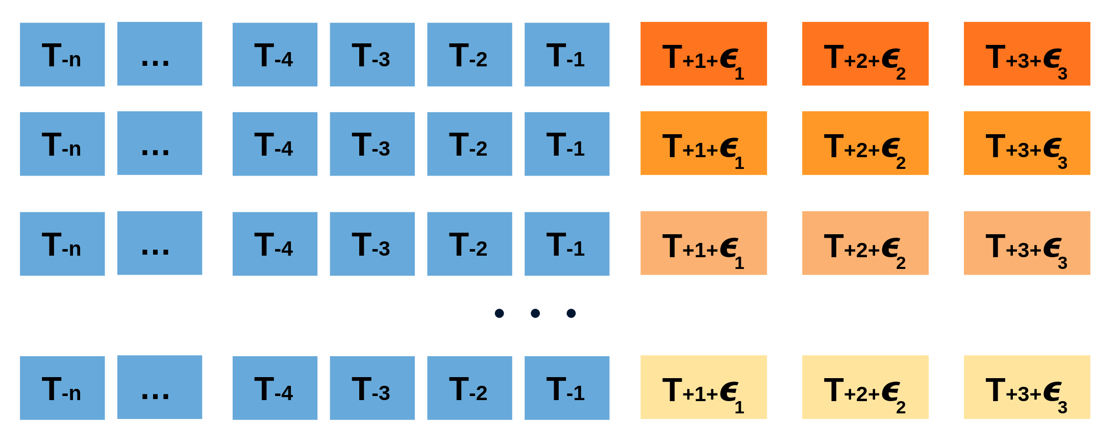
Bootstrapping predictions.
Using the outcome of the bootstrapping process, prediction intervals can be computed by calculating the $α/2$ and $1 − α/2$ percentiles at each forecasting horizon.
Animation of probabilistic bootstrapping prediction process.
Alternatively, it is also possible to fit a parametric distribution for each forecast horizon.
One of the main advantages of this strategy is that it requires only a single model to estimate any interval. However, performing hundreds or thousands of bootstrapping iterations can be computationally expensive and may not always be feasible.
Libraries and data
# Data processing
# ==============================================================================
import numpy as np
import pandas as pd
from skforecast.datasets import fetch_dataset
# Plots
# ==============================================================================
import matplotlib.pyplot as plt
import plotly.graph_objects as go
import plotly.io as pio
import plotly.offline as poff
pio.templates.default = "seaborn"
pio.renderers.default = 'notebook'
poff.init_notebook_mode(connected=True)
plt.style.use('seaborn-v0_8-darkgrid')
from skforecast.plot import plot_residuals
from pprint import pprint
# Modelling and Forecasting
# ==============================================================================
import skforecast
from lightgbm import LGBMRegressor
from sklearn.pipeline import make_pipeline
from feature_engine.datetime import DatetimeFeatures
from feature_engine.creation import CyclicalFeatures
from skforecast.recursive import ForecasterRecursive
from skforecast.direct import ForecasterDirect
from skforecast.preprocessing import RollingFeatures
from skforecast.model_selection import TimeSeriesFold, backtesting_forecaster, bayesian_search_forecaster
from skforecast.metrics import calculate_coverage, create_mean_pinball_loss
# Configuration
# ==============================================================================
import warnings
warnings.filterwarnings('once')
color = '\033[1m\033[38;5;208m'
print(f"{color}Version skforecast: {skforecast.__version__}")
Version skforecast: 0.22.0
# Data download
# ==============================================================================
data = fetch_dataset(name='bike_sharing', raw=False)
data = data[['users', 'temp', 'hum', 'windspeed', 'holiday']]
data = data.loc['2011-04-01 00:00:00':'2012-10-20 23:00:00', :].copy()
data.head(3)
╭───────────────────────────────── bike_sharing ──────────────────────────────────╮ │ Description: │ │ Hourly usage of the bike share system in the city of Washington D.C. during the │ │ years 2011 and 2012. In addition to the number of users per hour, information │ │ about weather conditions and holidays is available. │ │ │ │ Source: │ │ Fanaee-T,Hadi. (2013). Bike Sharing Dataset. UCI Machine Learning Repository. │ │ https://doi.org/10.24432/C5W894. │ │ │ │ URL: │ │ https://raw.githubusercontent.com/skforecast/skforecast- │ │ datasets/main/data/bike_sharing_dataset_clean.csv │ │ │ │ Shape: 17544 rows x 11 columns │ ╰─────────────────────────────────────────────────────────────────────────────────╯
| users | temp | hum | windspeed | holiday | |
|---|---|---|---|---|---|
| date_time | |||||
| 2011-04-01 00:00:00 | 6.0 | 10.66 | 100.0 | 11.0014 | 0.0 |
| 2011-04-01 01:00:00 | 4.0 | 10.66 | 100.0 | 11.0014 | 0.0 |
| 2011-04-01 02:00:00 | 7.0 | 10.66 | 93.0 | 12.9980 | 0.0 |
Additional features are created based on calendar information.
# Calendar features
# ==============================================================================
features_to_extract = ['month', 'week', 'day_of_week', 'hour']
calendar_transformer = DatetimeFeatures(
variables = 'index',
features_to_extract = features_to_extract,
drop_original = False,
)
# Cliclical encoding of calendar features
# ==============================================================================
features_to_encode = ['month', 'week', 'day_of_week', 'hour']
max_values = {"month": 12, "week": 52, "day_of_week": 7, "hour": 24}
cyclical_encoder = CyclicalFeatures(
variables = features_to_encode,
max_values = max_values,
drop_original = True
)
exog_transformer = make_pipeline(calendar_transformer, cyclical_encoder)
data = exog_transformer.fit_transform(data)
exog_features = data.columns.difference(['users']).tolist()
data.head(3)
| users | temp | hum | windspeed | holiday | month_sin | month_cos | week_sin | week_cos | day_of_week_sin | day_of_week_cos | hour_sin | hour_cos | |
|---|---|---|---|---|---|---|---|---|---|---|---|---|---|
| date_time | |||||||||||||
| 2011-04-01 00:00:00 | 6.0 | 10.66 | 100.0 | 11.0014 | 0.0 | 0.866025 | -0.5 | 1.0 | 6.123234e-17 | -0.433884 | -0.900969 | 0.000000 | 1.000000 |
| 2011-04-01 01:00:00 | 4.0 | 10.66 | 100.0 | 11.0014 | 0.0 | 0.866025 | -0.5 | 1.0 | 6.123234e-17 | -0.433884 | -0.900969 | 0.258819 | 0.965926 |
| 2011-04-01 02:00:00 | 7.0 | 10.66 | 93.0 | 12.9980 | 0.0 | 0.866025 | -0.5 | 1.0 | 6.123234e-17 | -0.433884 | -0.900969 | 0.500000 | 0.866025 |
To facilitate the training of the models, the search for optimal hyperparameters and the evaluation of their predictive accuracy, the data are divided into three separate sets: training, validation and test.
# Split train-validation-test
# ==============================================================================
end_train = '2012-06-30 23:59:00'
end_validation = '2012-10-01 23:59:00'
data_train = data.loc[: end_train, :]
data_val = data.loc[end_train:end_validation, :]
data_test = data.loc[end_validation:, :]
print(f"Dates train : {data_train.index.min()} --- {data_train.index.max()} (n={len(data_train)})")
print(f"Dates validacion : {data_val.index.min()} --- {data_val.index.max()} (n={len(data_val)})")
print(f"Dates test : {data_test.index.min()} --- {data_test.index.max()} (n={len(data_test)})")
Dates train : 2011-04-01 00:00:00 --- 2012-06-30 23:00:00 (n=10968) Dates validacion : 2012-07-01 00:00:00 --- 2012-10-01 23:00:00 (n=2232) Dates test : 2012-10-02 00:00:00 --- 2012-10-20 23:00:00 (n=456)
# Plot partitions
# ==============================================================================
fig = go.Figure()
fig.add_trace(go.Scatter(x=data_train.index, y=data_train['users'], mode='lines', name='Train'))
fig.add_trace(go.Scatter(x=data_val.index, y=data_val['users'], mode='lines', name='Validation'))
fig.add_trace(go.Scatter(x=data_test.index, y=data_test['users'], mode='lines', name='Test'))
fig.update_layout(
title='Number of users',
xaxis_title="Time",
yaxis_title="Users",
width=800,
height=400,
margin=dict(l=20, r=20, t=35, b=20),
legend=dict(orientation="h", yanchor="top", y=1, xanchor="left", x=0.001
)
)
fig.show()
Intervals with In-sample residuals
Intervals can be computed using in-sample residuals (residuals from the training set), either by calling the predict_interval() method, or by performing a full backtesting procedure. However, this can result in intervals that are too narrow (overly optimistic).
✏️ Note
Hyperparameters used in this example have been previously optimized using a bayesian search process. For more information about this process, please refer to Hyperparameter tuning and lags selection.
# Create and fit forecaster
# ==============================================================================
params = {
"max_depth": 7,
"n_estimators": 300,
"learning_rate": 0.06,
"verbose": -1,
"random_state": 15926
}
lags = [1, 2, 3, 23, 24, 25, 167, 168, 169]
window_features = RollingFeatures(stats=["mean"], window_sizes=24 * 3)
forecaster = ForecasterRecursive(
estimator = LGBMRegressor(**params),
lags = lags,
window_features = window_features,
)
forecaster.fit(
y = data.loc[:end_validation, 'users'],
exog = data.loc[:end_validation, exog_features],
store_in_sample_residuals = True
)
# In-sample residuals stored during fit
# ==============================================================================
print("Amount of residuals stored:", len(forecaster.in_sample_residuals_))
forecaster.in_sample_residuals_
Amount of residuals stored: 10000
array([ 42.02327339, -4.75342728, -39.26777553, ..., -3.54886809,
-41.20842177, -13.42207696])
The backtesting_forecaster() function is used to estimate the prediction intervals for the entire test set. Few arguments are required to use this function:
use_in_sample_residuals: IfTrue, the in-sample residuals are used to compute the prediction intervals. Since these residuals are obtained from the training set, they are always available, but usually lead to overoptimistic intervals. IfFalse, the out-sample residuals are used to calculate the prediction intervals. These residuals are obtained from the validation set and are only available if theset_out_sample_residuals()method has been called. It is recommended to use out-sample residuals to achieve the desired coverage.interval: the quantiles used to calculate the prediction intervals. For example, if the 10th and 90th percentiles are used, the resulting prediction intervals will have a nominal coverage of 80%.interval_method: the method used to calculate the prediction intervals. Available options arebootstrapingandconformal.n_boot: the number of bootstrap samples to be used in estimating the prediction intervals wheninterval_method='bootstraping'. The larger the number of samples, the more accurate the prediction intervals will be, but the longer the calculation will take.
# Backtesting with prediction intervals in test data using in-sample residuals
# ==============================================================================
cv = TimeSeriesFold(steps = 24, initial_train_size = len(data.loc[:end_validation]))
metric, predictions = backtesting_forecaster(
forecaster = forecaster,
y = data['users'],
exog = data[exog_features],
cv = cv,
metric = 'mean_absolute_error',
interval = [10, 90], # 80% prediction interval
interval_method = 'bootstrapping',
n_boot = 150,
use_in_sample_residuals = True, # Use in-sample residuals
use_binned_residuals = False,
)
predictions.head(5)
| fold | pred | lower_bound | upper_bound | |
|---|---|---|---|---|
| 2012-10-02 00:00:00 | 0 | 58.387527 | 32.799491 | 78.248425 |
| 2012-10-02 01:00:00 | 0 | 17.870302 | -7.253084 | 50.190172 |
| 2012-10-02 02:00:00 | 0 | 7.901576 | -17.057776 | 37.596425 |
| 2012-10-02 03:00:00 | 0 | 5.414332 | -16.809510 | 40.194483 |
| 2012-10-02 04:00:00 | 0 | 10.379630 | -12.696466 | 56.904041 |
# Function to plot predicted intervals
# ======================================================================================
def plot_predicted_intervals(
predictions: pd.DataFrame,
y_true: pd.DataFrame,
target_variable: str,
initial_x_zoom: list = None,
title: str = None,
xaxis_title: str = None,
yaxis_title: str = None,
):
"""
Plot predicted intervals vs real values
Parameters
----------
predictions : pandas DataFrame
Predicted values and intervals.
y_true : pandas DataFrame
Real values of target variable.
target_variable : str
Name of target variable.
initial_x_zoom : list, default `None`
Initial zoom of x-axis, by default None.
title : str, default `None`
Title of the plot, by default None.
xaxis_title : str, default `None`
Title of x-axis, by default None.
yaxis_title : str, default `None`
Title of y-axis, by default None.
"""
fig = go.Figure([
go.Scatter(name='Prediction', x=predictions.index, y=predictions['pred'], mode='lines'),
go.Scatter(name='Real value', x=y_true.index, y=y_true[target_variable], mode='lines'),
go.Scatter(
name='Upper Bound', x=predictions.index, y=predictions['upper_bound'],
mode='lines', marker=dict(color="#444"), line=dict(width=0), showlegend=False
),
go.Scatter(
name='Lower Bound', x=predictions.index, y=predictions['lower_bound'],
marker=dict(color="#444"), line=dict(width=0), mode='lines',
fillcolor='rgba(68, 68, 68, 0.3)', fill='tonexty', showlegend=False
)
])
fig.update_layout(
title=title, xaxis_title=xaxis_title, yaxis_title=yaxis_title, width=800,
height=400, margin=dict(l=20, r=20, t=35, b=20), hovermode="x",
xaxis=dict(range=initial_x_zoom),
legend=dict(orientation="h", yanchor="top", y=1.1, xanchor="left", x=0.001)
)
fig.show()
# Plot intervals
# ==============================================================================
plot_predicted_intervals(
predictions = predictions,
y_true = data_test,
target_variable = "users",
xaxis_title = "Date time",
yaxis_title = "users",
)
# Coverage (on test data)
# ==============================================================================
coverage = calculate_coverage(
y_true = data.loc[end_validation:, 'users'],
lower_bound = predictions["lower_bound"],
upper_bound = predictions["upper_bound"]
)
print(f"Predicted interval coverage: {round(100 * coverage, 2)} %")
# Area of the interval
# ==============================================================================
area = (predictions["upper_bound"] - predictions["lower_bound"]).sum()
print(f"Area of the interval: {round(area, 2)}")
Predicted interval coverage: 61.84 % Area of the interval: 43177.89
The prediction intervals exhibit overconfidence as they tend to be excessively narrow, resulting in a true coverage that falls below the nominal coverage. This phenomenon arises from the tendency of in-sample residuals to often overestimate the predictive capacity of the model.
# Store results for later comparison
# ==============================================================================
predictions_in_sample_residuals = predictions.copy()
Out-sample residuals (non-conditioned on predicted values)
To address the issue of overoptimistic intervals, it is possible to use out-sample residuals (residuals from a validation set not seen during training) to estimate the prediction intervals. These residuals can be obtained through backtesting.
# Backtesting on validation data to obtain out-sample residuals
# ==============================================================================
cv = TimeSeriesFold(steps = 24, initial_train_size = len(data.loc[:end_train]))
_, predictions_val = backtesting_forecaster(
forecaster = forecaster,
y = data.loc[:end_validation, 'users'],
exog = data.loc[:end_validation, exog_features],
cv = cv,
metric = 'mean_absolute_error',
)
# Out-sample residuals distribution
# ==============================================================================
residuals = data.loc[predictions_val.index, 'users'] - predictions_val['pred']
print(pd.Series(np.where(residuals < 0, 'negative', 'positive')).value_counts())
plt.rcParams.update({'font.size': 8})
_ = plot_residuals(residuals=residuals, figsize=(7, 4))
positive 1297 negative 935 Name: count, dtype: int64

With the set_out_sample_residuals() method, the out-sample residuals are stored in the forecaster object so that they can be used to calibrate the prediction intervals.
# Store out-sample residuals in the forecaster
# ==============================================================================
forecaster.set_out_sample_residuals(
y_true = data.loc[predictions_val.index, 'users'],
y_pred = predictions_val['pred']
)
Now that the new residuals have been added to the forecaster, the prediction intervals can be calculated using use_in_sample_residuals = False.
# Backtesting with prediction intervals in test data using out-sample residuals
# ==============================================================================
cv = TimeSeriesFold(steps = 24, initial_train_size = len(data.loc[:end_validation]))
metric, predictions = backtesting_forecaster(
forecaster = forecaster,
y = data['users'],
exog = data[exog_features],
cv = cv,
metric = 'mean_absolute_error',
interval = [10, 90], # 80% prediction interval
interval_method = 'bootstrapping',
n_boot = 150,
use_in_sample_residuals = False, # Use out-sample residuals
use_binned_residuals = False,
)
predictions.head(3)
| fold | pred | lower_bound | upper_bound | |
|---|---|---|---|---|
| 2012-10-02 00:00:00 | 0 | 58.387527 | 30.961801 | 133.296285 |
| 2012-10-02 01:00:00 | 0 | 17.870302 | -14.031592 | 132.635745 |
| 2012-10-02 02:00:00 | 0 | 7.901576 | -32.265023 | 142.360525 |
# Plot intervals
# ==============================================================================
plot_predicted_intervals(
predictions = predictions,
y_true = data_test,
target_variable = "users",
xaxis_title = "Date time",
yaxis_title = "users",
)
# Predicted interval coverage (on test data)
# ==============================================================================
coverage = calculate_coverage(
y_true = data.loc[end_validation:, 'users'],
lower_bound = predictions["lower_bound"],
upper_bound = predictions["upper_bound"]
)
print(f"Predicted interval coverage: {round(100 * coverage, 2)} %")
# Area of the interval
# ==============================================================================
area = (predictions["upper_bound"] - predictions["lower_bound"]).sum()
print(f"Area of the interval: {round(area, 2)}")
Predicted interval coverage: 83.33 % Area of the interval: 101257.22
The prediction intervals derived from the out-of-sample residuals are considerably wider than those based on the in-sample residuals, resulting in an empirical coverage closer to the nominal coverage. Looking at the plot, it's clear that the intervals are particularly wide at low predicted values, suggesting that the model struggles to accurately capture the uncertainty in its predictions at these lower values.
# Store results for later comparison
# ==============================================================================
predictions_out_sample_residuals = predictions.copy()
Intervals conditioned on predicted values (binned residuals)
The bootstrapping process assumes that the residuals are independently distributed so that they can be used independently of the predicted value. In reality, this is rarely true; in most cases, the magnitude of the residuals is correlated with the magnitude of the predicted value. In this case, for example, one would hardly expect the error to be the same when the predicted number of users is close to zero as when it is in the hundreds.
To account for the dependence between the residuals and the predicted values, skforecast allows to partition the residuals into K bins, where each bin is associated with a range of predicted values. Using this strategy, the bootstrapping process samples the residuals from different bins depending on the predicted value, which can improve the coverage of the interval while adjusting the width if necessary, allowing the model to better distribute the uncertainty of its predictions.
Internally, skforecast uses a QuantileBinner class to bin data into quantile-based bins using numpy.percentile. This class is similar to KBinsDiscretizer but faster for binning data into quantile-based bins. Bin intervals are defined following the convention: bins[i-1] <= x < bins[i]. The binning process can be adjusted using the argument binner_kwargs of the Forecaster object.
# Create and train forecaster
# ==============================================================================
forecaster = ForecasterRecursive(
estimator = LGBMRegressor(**params),
lags = lags,
binner_kwargs = {'n_bins': 5}
)
forecaster.fit(
y = data.loc[:end_validation, 'users'],
exog = data.loc[:end_validation, exog_features],
store_in_sample_residuals = True
)
During the training process, the forecaster uses the in-sample predictions to define the intervals at which the residuals are stored depending on the predicted value to which they are related (binner_intervals_ attribute). For example, if the bin "0" has an interval of (5.5, 10.7), it means that it will store the residuals of the predictions that fall within that interval.
When the prediction intervals are calculated, the residuals are sampled from the bin corresponding to the predicted value. This way, the model can adjust the width of the intervals depending on the predicted value, which can help to better distribute the uncertainty of the predictions.
# Intervals associated with the bins
# ==============================================================================
pprint(forecaster.binner_intervals_)
{0: (-0.8943794883271247, 30.676160623625577),
1: (30.676160623625577, 120.49652689276296),
2: (120.49652689276296, 209.69596300954962),
3: (209.69596300954962, 338.3331511270013),
4: (338.3331511270013, 955.802117392104)}
The set_out_sample_residuals() method will bin the residuals according to the intervals learned during fitting. To avoid using too much memory, the number of residuals stored per bin is limited to 10_000 // self.binner.n_bins_.
# Store out-sample residuals in the forecaster
# ==============================================================================
forecaster.set_out_sample_residuals(
y_true = data.loc[predictions_val.index, 'users'],
y_pred = predictions_val['pred']
)
# Number of out-sample residuals by bin
# ==============================================================================
for k, v in forecaster.out_sample_residuals_by_bin_.items():
print(f"Bin {k}: n={len(v)}")
Bin 0: n=321 Bin 1: n=315 Bin 2: n=310 Bin 3: n=534 Bin 4: n=752
# Distribution of the residual by bin
# ==============================================================================
out_sample_residuals_by_bin_df = pd.DataFrame(
dict(
[(k, pd.Series(v))
for k, v in forecaster.out_sample_residuals_by_bin_.items()]
)
)
fig, ax = plt.subplots(figsize=(6, 3))
out_sample_residuals_by_bin_df.boxplot(ax=ax)
ax.set_title("Distribution of residuals by bin", fontsize=12)
ax.set_xlabel("Bin", fontsize=10)
ax.set_ylabel("Residuals", fontsize=10)
plt.show();

The box plots show how the spread and magnitude of the residuals differ depending on the predicted value. The residuals are higher and more dispersed when the predicted value is higher (higer bin), which is consistent with the intuition that errors tend to be larger when the predicted value is larger.
# Summary information of bins
# ======================================================================================
bins_summary = {
key: pd.DataFrame(value).describe().T.assign(bin=key)
for key, value
in forecaster.out_sample_residuals_by_bin_.items()
}
bins_summary = pd.concat(bins_summary.values()).set_index("bin")
bins_summary.insert(0, "interval", bins_summary.index.map(forecaster.binner_intervals_))
bins_summary['interval'] = bins_summary['interval'].apply(lambda x: np.round(x, 2))
bins_summary
| interval | count | mean | std | min | 25% | 50% | 75% | max | |
|---|---|---|---|---|---|---|---|---|---|
| bin | |||||||||
| 0 | [-0.89, 30.68] | 321.0 | 1.113833 | 12.168815 | -19.168802 | -4.060555 | -0.435406 | 3.392902 | 150.505840 |
| 1 | [30.68, 120.5] | 315.0 | 1.560517 | 31.195637 | -77.399525 | -13.424717 | -3.511859 | 10.819653 | 356.446585 |
| 2 | [120.5, 209.7] | 310.0 | 17.209087 | 51.763411 | -147.240066 | -7.478638 | 15.740146 | 38.113001 | 300.170968 |
| 3 | [209.7, 338.33] | 534.0 | 14.883687 | 69.231176 | -241.322880 | -18.266984 | 10.051186 | 42.654985 | 464.619346 |
| 4 | [338.33, 955.8] | 752.0 | 18.740171 | 105.830048 | -485.278643 | -23.429556 | 25.356507 | 77.634913 | 382.818946 |
Finally, the prediction intervals estimated again, this time using out-sample residuals conditioned on the predicted values.
# Backtesting with prediction intervals in test data using out-sample residuals
# ==============================================================================
cv = TimeSeriesFold(steps = 24, initial_train_size = len(data.loc[:end_validation]))
metric, predictions = backtesting_forecaster(
forecaster = forecaster,
y = data['users'],
exog = data[exog_features],
cv = cv,
metric = 'mean_absolute_error',
interval = [10, 90], # 80% prediction interval
interval_method = 'bootstrapping',
n_boot = 150,
use_in_sample_residuals = False, # Use out-sample residuals
use_binned_residuals = True, # Residuals conditioned on predicted values
)
predictions.head(3)
| fold | pred | lower_bound | upper_bound | |
|---|---|---|---|---|
| 2012-10-02 00:00:00 | 0 | 60.399647 | 38.496874 | 92.876947 |
| 2012-10-02 01:00:00 | 0 | 17.617464 | 9.065502 | 43.844047 |
| 2012-10-02 02:00:00 | 0 | 9.002365 | -0.636921 | 26.285576 |
# Plot intervals
# ==============================================================================
plot_predicted_intervals(
predictions = predictions,
y_true = data_test,
target_variable = "users",
xaxis_title = "Date time",
yaxis_title = "users",
)
# Predicted interval coverage (on test data)
# ==============================================================================
coverage = calculate_coverage(
y_true = data.loc[end_validation:, 'users'],
lower_bound = predictions["lower_bound"],
upper_bound = predictions["upper_bound"]
)
print(f"Predicted interval coverage: {round(100 * coverage, 2)} %")
# Area of the interval
# ==============================================================================
area = (predictions["upper_bound"] - predictions["lower_bound"]).sum()
print(f"Area of the interval: {round(area, 2)}")
Predicted interval coverage: 86.4 % Area of the interval: 95072.24
When using out-sample residuals conditioned on the predicted value, the area of the interval is significantly reduced and the uncertainty is mainly allocated to the predictions with high values. However, the empirical coverage is still above the expected coverage, which means that the estimated intervals are conservative.
The following plot compares the prediction intervals obtained using in-sample residuals, out-sample residuals, and out-sample residuals conditioned on the predicted values.
# Plot intervals using: in-sample residuals, out-sample residuals and binned residuals
# ==============================================================================
predictions_out_sample_residuals_binned = predictions.copy()
fig, ax = plt.subplots(figsize=(8, 4))
ax.fill_between(
data_test.index,
predictions_out_sample_residuals["lower_bound"],
predictions_out_sample_residuals["upper_bound"],
color='gray',
alpha=0.9,
label='Out-sample residuals',
zorder=1
)
ax.fill_between(
data_test.index,
predictions_out_sample_residuals_binned["lower_bound"],
predictions_out_sample_residuals_binned["upper_bound"],
color='#fc4f30',
alpha=0.7,
label='Out-sample binned residuals',
zorder=2
)
ax.fill_between(
data_test.index,
predictions_in_sample_residuals["lower_bound"],
predictions_in_sample_residuals["upper_bound"],
color='#30a2da',
alpha=0.9,
label='In-sample residuals',
zorder=3
)
ax.set_xlim(pd.to_datetime(["2012-10-08 00:00:00", "2012-10-15 00:00:00"]))
ax.set_title("Prediction intervals with different residuals", fontsize=12)
ax.legend();

⚠️ Warning
Probabilistic forecasting in production
The correct estimation of prediction intervals depends on the residuals being representative of future errors. For this reason, out-of-sample residuals should be used. However, the dynamics of the series and models can change over time, so it is important to monitor and regularly update the residuals. It can be done easily using the set_out_sample_residuals() method.
Prediction of multiple intervals
The backtesting_forecaster function not only allows to estimate a single prediction interval, but also to estimate multiple quantiles (percentiles) from which multiple prediction intervals can be constructed. This is useful to evaluate the quality of the prediction intervals for a range of probabilities. Furthermore, it has almost no additional computational cost compared to estimating a single interval.
Next, several percentiles are predicted and from these, prediction intervals are created for different nominal coverage levels - 10%, 20%, 30%, 40%, 50%, 60%, 70%, 80%, 90% and 95% - and their actual coverage is assessed.
# Prediction intervals for different nominal coverages
# ==============================================================================
quantiles = [2.5, 5, 10, 15, 20, 25, 30, 35, 40, 45, 50, 55, 60, 65, 70, 75, 80, 85, 90, 95, 97.5]
intervals = [[2.5, 97.5], [5, 95], [10, 90], [15, 85], [20, 80], [30, 70], [35, 65], [40, 60], [45, 55]]
observed_coverages = []
observed_areas = []
metric, predictions = backtesting_forecaster(
forecaster = forecaster,
y = data['users'],
exog = data[exog_features],
cv = cv,
metric = 'mean_absolute_error',
interval = quantiles,
interval_method = 'bootstrapping',
n_boot = 150,
use_in_sample_residuals = False, # Use out-sample residuals
use_binned_residuals = True
)
predictions.head()
| fold | pred | p_2.5 | p_5 | p_10 | p_15 | p_20 | p_25 | p_30 | p_35 | ... | p_55 | p_60 | p_65 | p_70 | p_75 | p_80 | p_85 | p_90 | p_95 | p_97.5 | |
|---|---|---|---|---|---|---|---|---|---|---|---|---|---|---|---|---|---|---|---|---|---|
| 2012-10-02 00:00:00 | 0 | 60.399647 | 26.540465 | 32.237144 | 38.496874 | 42.515102 | 46.248204 | 48.730080 | 49.747541 | 50.830767 | ... | 59.877370 | 61.388407 | 63.572870 | 66.179578 | 70.417796 | 77.232456 | 82.866190 | 92.876947 | 109.483516 | 118.113906 |
| 2012-10-02 01:00:00 | 0 | 17.617464 | 4.028027 | 6.993912 | 9.065502 | 10.218569 | 11.732744 | 13.290492 | 15.065701 | 15.542016 | ... | 19.700862 | 21.330240 | 22.453599 | 25.298972 | 28.853490 | 32.110319 | 35.993433 | 43.844047 | 68.261638 | 77.072027 |
| 2012-10-02 02:00:00 | 0 | 9.002365 | -5.454406 | -2.921308 | -0.636921 | 2.627889 | 4.072849 | 5.556213 | 6.372106 | 7.170950 | ... | 11.673119 | 12.670580 | 14.060076 | 15.750417 | 17.660921 | 19.929581 | 23.416450 | 26.285576 | 41.378533 | 52.759679 |
| 2012-10-02 03:00:00 | 0 | 5.306644 | -7.830956 | -6.205384 | -1.102749 | -0.500265 | 1.101968 | 2.283863 | 3.161327 | 4.006352 | ... | 6.650199 | 7.561984 | 8.280507 | 9.689953 | 10.880484 | 11.786155 | 14.400937 | 17.854639 | 24.489084 | 41.218966 |
| 2012-10-02 04:00:00 | 0 | 9.439573 | -6.712543 | -2.292124 | 3.206393 | 5.276201 | 5.718478 | 6.576003 | 7.203672 | 8.176026 | ... | 11.509308 | 12.074734 | 12.427330 | 13.552448 | 14.515979 | 15.536160 | 17.744162 | 22.566557 | 27.379155 | 53.829421 |
5 rows × 23 columns
# Calculate coverage and area for each interval
# ==============================================================================
for interval in intervals:
observed_coverage = calculate_coverage(
y_true = data.loc[end_validation:, 'users'],
lower_bound = predictions[f"p_{interval[0]}"],
upper_bound = predictions[f"p_{interval[1]}"]
)
observed_area = (predictions[f"p_{interval[1]}"] - predictions[f"p_{interval[0]}"]).sum()
observed_coverages.append(100 * observed_coverage)
observed_areas.append(observed_area)
results = pd.DataFrame({
'Interval': intervals,
'Nominal coverage': [interval[1] - interval[0] for interval in intervals],
'Observed coverage': observed_coverages,
'Area': observed_areas
})
results.round(1)
| Interval | Nominal coverage | Observed coverage | Area | |
|---|---|---|---|---|
| 0 | [2.5, 97.5] | 95.0 | 96.7 | 163585.0 |
| 1 | [5, 95] | 90.0 | 93.4 | 129723.9 |
| 2 | [10, 90] | 80.0 | 86.4 | 95072.2 |
| 3 | [15, 85] | 70.0 | 79.8 | 73890.3 |
| 4 | [20, 80] | 60.0 | 74.1 | 58018.5 |
| 5 | [30, 70] | 40.0 | 51.1 | 34447.4 |
| 6 | [35, 65] | 30.0 | 40.6 | 24832.8 |
| 7 | [40, 60] | 20.0 | 26.5 | 16087.9 |
| 8 | [45, 55] | 10.0 | 12.5 | 8026.3 |
Predict boostrap, interval, quantile and distribution
The previous sections have demonstrated the use of the backtesting process to estimate the prediction interval over a given period of time. The goal is to mimic the behavior of the model in production by running predictions at regular intervals, incrementally updating the input data.
Alternatively, it is possible to run a single prediction that forecasts N steps ahead without going through the entire backtesting process. In such cases, skforecast provides four different methods: predict_bootstrapping, predict_interval, predict_quantile and predict_dist. For detailed information on how to use these methods, please refer to the documentation.
Conformal Prediction
Conformal prediction is a framework for constructing prediction intervals that are guaranteed to contain the true value with a specified probability (coverage probability). It works by combining the predictions of a point-forecasting model with its past residuals—differences between previous predictions and actual values. These residuals help estimate the uncertainty in the forecast and determine the width of the prediction interval that is then added to the point forecast. Skforecast implements Split Conformal Prediction (SCP).
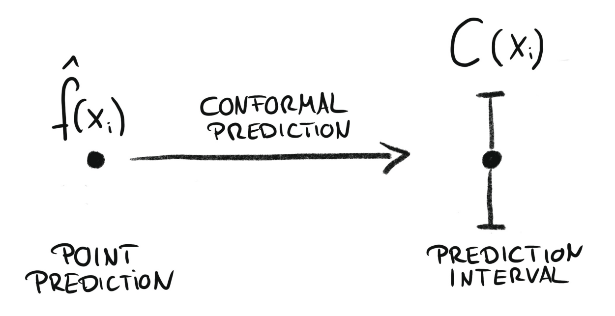
Conformal regression turns point predictions into prediction intervals. Source: Introduction To Conformal Prediction With Python: A Short Guide For Quantifying Uncertainty Of Machine Learning Models
by Christoph Molnar https://leanpub.com/conformal-prediction
Animation of probabilistic conformal prediction process.
Conformal methods can also calibrate prediction intervals generated by other techniques, such as quantile regression or bootstrapped residuals. In this case, the conformal method adjusts the prediction intervals to ensure that they remain valid with respect to the coverage probability. Skforecast provides this functionality through the ConformalIntervalCalibrator transformer.
⚠️ Warning
There are several well-established methods for conformal prediction, each with its own characteristics and assumptions. However, when applied to time series forecasting, their coverage guarantees are only valid for one-step-ahead predictions. For multi-step-ahead predictions, the coverage probability is not guaranteed. Skforecast implements Split Conformal Prediction (SCP) due to its balance between complexity and performance.
A backtesting process is applied to estimate the prediction intervals for the test set, this time using the conformal method. Since the outsample residuals are already stored in the forecaster object, the use_in_sample_residuals argument is set to False, and use_binned_residuals is set to True to allow adaptive intervals.
# Backtesting with prediction intervals in test data using out-sample residuals
# ==============================================================================
cv = TimeSeriesFold(steps = 24, initial_train_size = len(data.loc[:end_validation]))
metric, predictions = backtesting_forecaster(
forecaster = forecaster,
y = data['users'],
exog = data[exog_features],
cv = cv,
metric = 'mean_absolute_error',
interval = 0.8, # 80% prediction interval
interval_method = 'conformal',
use_in_sample_residuals = False, # Use out-sample residuals
use_binned_residuals = True, # Adaptive conformal
)
predictions.head(3)
| fold | pred | lower_bound | upper_bound | |
|---|---|---|---|---|
| 2012-10-02 00:00:00 | 0 | 60.399647 | 32.785300 | 88.013993 |
| 2012-10-02 01:00:00 | 0 | 17.617464 | 8.692943 | 26.541985 |
| 2012-10-02 02:00:00 | 0 | 9.002365 | 0.077843 | 17.926886 |
# Plot intervals
# ==============================================================================
plot_predicted_intervals(
predictions = predictions,
y_true = data_test,
target_variable = "users",
xaxis_title = "Date time",
yaxis_title = "users",
)
# Predicted interval coverage (on test data)
# ==============================================================================
coverage = calculate_coverage(
y_true = data.loc[end_validation:, 'users'],
lower_bound = predictions["lower_bound"],
upper_bound = predictions["upper_bound"]
)
print(f"Predicted interval coverage: {round(100 * coverage, 2)} %")
# Area of the interval
# ==============================================================================
area = (predictions["upper_bound"] - predictions["lower_bound"]).sum()
print(f"Area of the interval: {round(area, 2)}")
Predicted interval coverage: 78.29 % Area of the interval: 64139.13
The resulting intervals show a slightly lower coverage than the expected 80%, but close to it.
Quantile Regression
Quantile regression is a technique for estimating the conditional quantiles of a response variable. By combining the predictions of two quantile regressors, an interval can be constructed, where each model estimates one of the interval’s boundaries. For example, models trained for $Q = 0.1$ and $Q = 0.9$ produce an 80% prediction interval ($90\% - 10\% = 80\%$).
If a machine learning algorithm capable of modeling quantiles is used as the estimator in a forecaster, the predict method will return predictions for a specified quantile. By creating two forecasters, each configured with a different quantile, their predictions can be combined to generate a prediction interval.
As opposed to linear regression, which is intended to estimate the conditional mean of the response variable given certain values of the predictor variables, quantile regression aims at estimating the conditional quantiles of the response variable. For a continuous distribution function, the $\alpha$-quantile $Q_{\alpha}(x)$ is defined such that the probability of $Y$ being smaller than $Q_{\alpha}(x)$ is, for a given $X=x$, equal to $\alpha$. For example, 36% of the population values are lower than the quantile $Q=0.36$. The most known quantile is the 50%-quantile, more commonly called the median.
By combining the predictions of two quantile regressors, it is possible to build an interval. Each model estimates one of the limits of the interval. For example, the models obtained for $Q = 0.1$ and $Q = 0.9$ produce an 80% prediction interval (90% - 10% = 80%).
Several machine learning algorithms are capable of modeling quantiles. Some of them are:
Just as the squared-error loss function is used to train models that predict the mean value, a specific loss function is needed in order to train models that predict quantiles. The most common metric used for quantile regression is called quantile loss or pinball loss:
$$\text{pinball}(y, \hat{y}) = \frac{1}{n_{\text{samples}}} \sum_{i=0}^{n_{\text{samples}}-1} \alpha \max(y_i - \hat{y}_i, 0) + (1 - \alpha) \max(\hat{y}_i - y_i, 0)$$where $\alpha$ is the target quantile, $y$ the real value and $\hat{y}$ the quantile prediction.
It can be seen that loss differs depending on the evaluated quantile. The higher the quantile, the more the loss function penalizes underestimates, and the less it penalizes overestimates. As with MSE and MAE, the goal is to minimize its values (the lower loss, the better).
Two disadvantages of quantile regression, compared to the bootstrap approach to prediction intervals, are that each quantile needs its estimator and quantile regression is not available for all types of regression models. However, once the models are trained, the inference is much faster since no iterative process is needed.
This type of prediction intervals can be easily estimated using ForecasterDirect and ForecasterDirectMultiVariate models.
⚠️ Warning
Forecasters of type ForecasterDirect are slower than ForecasterRecursive because they require training one model per step. Although they can achieve better performance, their scalability is an important limitation when many steps need to be predicted.
# Create forecasters: one for each limit of the interval
# ==============================================================================
# The forecasters obtained for alpha=0.1 and alpha=0.9 produce a 80% confidence
# interval (90% - 10% = 80%).
# Forecaster for quantile 10%
forecaster_q10 = ForecasterDirect(
estimator = LGBMRegressor(
objective = 'quantile',
metric = 'quantile',
alpha = 0.1,
random_state = 15926,
verbose = -1
),
lags = lags,
steps = 24
)
# Forecaster for quantile 90%
forecaster_q90 = ForecasterDirect(
estimator = LGBMRegressor(
objective = 'quantile',
metric = 'quantile',
alpha = 0.9,
random_state = 15926,
verbose = -1
),
lags = lags,
steps = 24
)
Next, a bayesian search is performed to find the best hyperparameters for the quantile regressors. When validating a quantile regression model, it is important to use a metric that is coherent with the quantile being evaluated. In this case, the pinball loss is used. Skforecast provides the function create_mean_pinball_loss calculate the pinball loss for a given quantile.
# Bayesian search of hyper-parameters and lags for each quantile forecaster
# ==============================================================================
def search_space(trial):
search_space = {
'n_estimators' : trial.suggest_int('n_estimators', 100, 500, step=50),
'max_depth' : trial.suggest_int('max_depth', 3, 10, step=1),
'learning_rate' : trial.suggest_float('learning_rate', 0.01, 0.1)
}
return search_space
cv = TimeSeriesFold(steps = 24, initial_train_size = len(data[:end_train]))
results_grid_q10 = bayesian_search_forecaster(
forecaster = forecaster_q10,
y = data.loc[:end_validation, 'users'],
cv = cv,
metric = create_mean_pinball_loss(alpha=0.1),
search_space = search_space,
n_trials = 10
)
results_grid_q90 = bayesian_search_forecaster(
forecaster = forecaster_q90,
y = data.loc[:end_validation, 'users'],
cv = cv,
metric = create_mean_pinball_loss(alpha=0.9),
search_space = search_space,
n_trials = 10
)
Once the best hyper-parameters have been found for each forecaster, a backtesting process is applied again using the test data.
# Backtesting on test data
# ==============================================================================
cv = TimeSeriesFold(steps = 24, initial_train_size = len(data.loc[:end_validation]))
metric_q10, predictions_q10 = backtesting_forecaster(
forecaster = forecaster_q10,
y = data['users'],
cv = cv,
metric = create_mean_pinball_loss(alpha=0.1)
)
metric_q90, predictions_q90 = backtesting_forecaster(
forecaster = forecaster_q90,
y = data['users'],
cv = cv,
metric = create_mean_pinball_loss(alpha=0.9)
)
predictions = pd.concat([predictions_q10['pred'], predictions_q90['pred']], axis=1)
predictions.columns = ['lower_bound', 'upper_bound']
predictions.head(3)
| lower_bound | upper_bound | |
|---|---|---|
| 2012-10-02 00:00:00 | 39.108177 | 73.136230 |
| 2012-10-02 01:00:00 | 11.837010 | 32.588538 |
| 2012-10-02 02:00:00 | 4.453201 | 14.346566 |
# Plot
# ==============================================================================
fig = go.Figure([
go.Scatter(name='Real value', x=data_test.index, y=data_test['users'], mode='lines'),
go.Scatter(
name='Upper Bound', x=predictions.index, y=predictions['upper_bound'],
mode='lines', marker=dict(color="#444"), line=dict(width=0), showlegend=False
),
go.Scatter(
name='Lower Bound', x=predictions.index, y=predictions['lower_bound'],
marker=dict(color="#444"), line=dict(width=0), mode='lines',
fillcolor='rgba(68, 68, 68, 0.3)', fill='tonexty', showlegend=False
)
])
fig.update_layout(
title="Real value vs predicted in test data",
xaxis_title="Date time",
yaxis_title="users",
width=800,
height=400,
margin=dict(l=20, r=20, t=35, b=20),
hovermode="x",
legend=dict(orientation="h", yanchor="top", y=1.1, xanchor="left", x=0.001)
)
fig.show()
# Predicted interval coverage (on test data)
# ==============================================================================
coverage = calculate_coverage(
y_true = data.loc[end_validation:, 'users'],
lower_bound = predictions["lower_bound"],
upper_bound = predictions["upper_bound"]
)
print(f"Predicted interval coverage: {round(100 * coverage, 2)} %")
# Area of the interval
# ==============================================================================
area = (predictions["upper_bound"] - predictions["lower_bound"]).sum()
print(f"Area of the interval: {round(area, 2)}")
Predicted interval coverage: 62.28 % Area of the interval: 109062.92
In this case, the quantile forecasting strategy does not achieve empirical coverage close to the expected coverage (80 percent).
External calibration of prediction intervals
It is frequent that the prediction intervals obtained with the different methods do not achieve the desired coverage because they are under or overconfident. To address this issue, skforecast provides the ConformalIntervalCalibrator, transformer, which can be used to calibrate the prediction intervals obtained with other methods.
Session information
import session_info
session_info.show(html=False)
----- feature_engine 1.9.4 lightgbm 4.6.0 matplotlib 3.10.8 numpy 2.1.3 pandas 2.3.3 plotly 6.6.0 session_info v1.0.1 skforecast 0.22.0 sklearn 1.7.2 ----- IPython 9.11.0 jupyter_client 8.8.0 jupyter_core 5.9.1 ----- Python 3.13.12 | packaged by Anaconda, Inc. | (main, Feb 24 2026, 16:13:31) [GCC 14.3.0] Linux-5.15.0-1084-aws-x86_64-with-glibc2.31 ----- Session information updated at 2026-04-23 12:43
Citation
How to cite this document
If you use this document or any part of it, please acknowledge the source, thank you!
Probabilistic forecasting with machine learning by Joaquín Amat Rodrigo and Javier Escobar Ortiz, available under Attribution-NonCommercial-ShareAlike 4.0 International (CC BY-NC-SA 4.0 DEED) at https://cienciadedatos.net/documentos/py42-probabilistic-forecasting.html
How to cite skforecast
If you use skforecast for a publication, we would appreciate if you cite the published software.
Zenodo:
Amat Rodrigo, Joaquin, & Escobar Ortiz, Javier. (2024). skforecast (v0.20.0). Zenodo. https://doi.org/10.5281/zenodo.8382788
APA:
Amat Rodrigo, J., & Escobar Ortiz, J. (2024). skforecast (Version 0.20.0) [Computer software]. https://doi.org/10.5281/zenodo.8382788
BibTeX:
@software{skforecast, author = {Amat Rodrigo, Joaquin and Escobar Ortiz, Javier}, title = {skforecast}, version = {0.20.0}, month = {01}, year = {2026}, license = {BSD-3-Clause}, url = {https://skforecast.org/}, doi = {10.5281/zenodo.8382788} }
Did you like the article? Your support is important
Your contribution will help me to continue generating free educational content. Many thanks! 😊


This work by Joaquín Amat Rodrigo and Javier Escobar Ortiz is licensed under a Attribution-NonCommercial-ShareAlike 4.0 International.
Allowed:
-
Share: copy and redistribute the material in any medium or format.
-
Adapt: remix, transform, and build upon the material.
Under the following terms:
-
Attribution: You must give appropriate credit, provide a link to the license, and indicate if changes were made. You may do so in any reasonable manner, but not in any way that suggests the licensor endorses you or your use.
-
NonCommercial: You may not use the material for commercial purposes.
-
ShareAlike: If you remix, transform, or build upon the material, you must distribute your contributions under the same license as the original.