更多关于时间序列预测,参见 cienciadedatos.net
- 使用 Python 的 ARIMA 与 SARIMAX 模型
- 使用机器学习进行时间序列预测
- 基于梯度提升的时间序列预测:XGBoost、LightGBM 与 CatBoost
- 使用 XGBoost 进行时间序列预测
- 全局预测模型:多序列预测
- 全局预测模型:单序列与多序列建模的对比分析
- 概率预测
- 用深度学习进行预测
- 使用机器学习预测能源需求
- 使用机器学习预测网站流量
- 间歇性需求预测
- 用树模型刻画时间序列趋势
- 用 Python 预测比特币价格
- 通过模型集成(Stacking)提升预测效果
- 可解释的预测模型
- 缓解 Covid 对预测模型的影响
- 含缺失值的时间序列预测

介绍
时间序列是按时间顺序排列的一组数据,采样间隔可以相等,也可以不相等。预测过程是指预测时间序列的未来值,这种建模方式可以仅依赖于序列自身的历史行为(自回归模型),也可以结合其他外部变量。
本指南将探讨如何使用 scikit-learn 回归模型来进行时间序列预测。具体来说,我们将介绍 skforecast,这是一个直观易用的库,提供了一系列核心类和函数,能够将任意 Scikit-learn 回归模型灵活调整,以有效解决预测相关的问题。
✏️ Note
本文档作为使用 skforecast 进行基于机器学习的预测入门指南。如需更高级和更详细的示例,请参阅 [skforecast 文档](https://skforecast.org/)。
用于时间序列预测的机器学习
为了将机器学习模型应用于预测问题,需要把时间序列转换为一个矩阵,使得每个值都与其之前的时间窗口(滞后项,lags)相关联。
在时间序列的语境中,相对于时刻 t 的滞后量(lag)被定义为序列在之前时刻的取值。例如,lag 1 是时刻 t−1 的值,而 lag m 是时刻 t−m 的值。
![]()
这种转换也允许加入额外的变量。
![]()
一旦将数据重排为上述形状,就可以训练任意回归模型来预测序列的下一个值(下一步)。在训练过程中,每一行都被视为一个独立样本,其中滞后 1、2、...、p 的取值作为特征,用于预测时间步 t+1 的目标值。
多步时间序列预测
在时间序列任务中,很少只需要预测下一个值(t{+1})。更常见的目标是预测一个未来区间((t{+1}), ..., (t{+n})),或某个更远的时间点(t{+n})。为此可以采用多种策略来生成这种类型的预测。
递归式多步预测
由于预测 tn 需要用到 t{n-1},而 t_{n-1} 在预测时未知,因此采用递归式过程:每一个新预测都以前一个预测为基础。这一过程称为递归式预测(recursive forecasting)或递归式多步预测,可通过 ForecasterRecursive 类轻松实现。


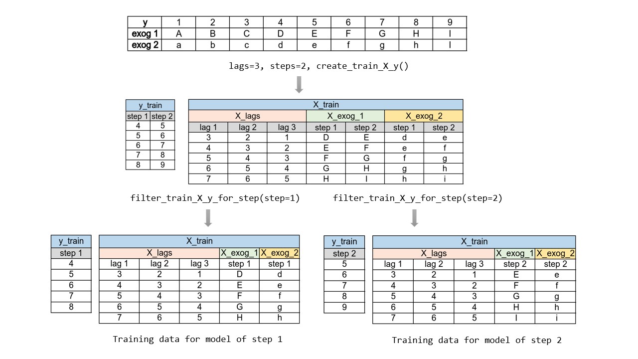
直接式多步预测
直接式多步预测(direct multi-step forecasting)为预测区间中的每一个步长训练一个独立模型。例如,要预测时间序列的未来 5 个取值,就要训练 5 个不同的模型,每个模型专注于其中一个步长。因此,不同步长上的预测彼此独立。


该方法的主要复杂性在于需要为每个步长生成正确的训练矩阵。skforecast 库中的 ForecasterDirect 类可将这一过程自动化。此外需要注意,此策略的计算成本更高,因为需要训练多个模型。下图展示了当响应变量与两个外生变量均可用时的处理流程。
多输出预测
某些机器学习模型(例如长短期记忆网络,LSTM)可以一次性(one-shot)同时预测序列的多个值。skforecast 库在 ForecasterRnn 类中实现了这种策略。
依赖库
本指南所用到的主要依赖如下:
# 数据处理
# ==============================================================================
import numpy as np
import pandas as pd
from skforecast.datasets import fetch_dataset
# 绘图
# ==============================================================================
import matplotlib.pyplot as plt
from skforecast.plot import set_dark_theme
# 建模与预测
# ==============================================================================
import sklearn
from sklearn.linear_model import Ridge
from sklearn.ensemble import RandomForestRegressor
from sklearn.metrics import mean_squared_error, mean_absolute_error
from sklearn.preprocessing import StandardScaler
import skforecast
from skforecast.recursive import ForecasterRecursive
from skforecast.direct import ForecasterDirect
from skforecast.model_selection import TimeSeriesFold, grid_search_forecaster, backtesting_forecaster
from skforecast.preprocessing import RollingFeatures
from skforecast.utils import save_forecaster, load_forecaster
from skforecast.metrics import calculate_coverage
from skforecast.plot import plot_prediction_intervals
import shap
# 警告配置
# ==============================================================================
import warnings
warnings.filterwarnings('once')
color = '\033[1m\033[38;5;208m'
print(f"{color}版本 skforecast: {skforecast.__version__}")
print(f"{color}版本 scikit-learn: {sklearn.__version__}")
print(f"{color}版本 pandas: {pd.__version__}")
print(f"{color}版本 numpy: {np.__version__}")
版本 skforecast: 0.22.0 版本 scikit-learn: 1.7.2 版本 pandas: 2.3.3 版本 numpy: 2.1.3
数据
本例提供了一条时间序列,表示 1991–2008 年间澳大利亚公共医疗系统在皮质类固醇药物上的每月支出(单位:百万美元)。我们的目标是创建一个自回归模型来预测未来的月度支出。本文所用数据来自经典教材 Forecasting: Principles and Practice by Rob J Hyndman and George Athanasopoulos。
# 数据下载
# ==============================================================================
data = fetch_dataset(name='h2o_exog', raw=True)
╭─────────────────────────────────── h2o_exog ────────────────────────────────────╮ │ Description: │ │ Monthly expenditure ($AUD) on corticosteroid drugs that the Australian health │ │ system had between 1991 and 2008. Two additional variables (exog_1, exog_2) are │ │ simulated. │ │ │ │ Source: │ │ Hyndman R (2023). fpp3: Data for Forecasting: Principles and Practice (3rd │ │ Edition). http://pkg.robjhyndman.com/fpp3package/, │ │ https://github.com/robjhyndman/fpp3package, http://OTexts.com/fpp3. │ │ │ │ URL: │ │ https://raw.githubusercontent.com/skforecast/skforecast- │ │ datasets/main/data/h2o_exog.csv │ │ │ │ Shape: 195 rows x 4 columns │ ╰─────────────────────────────────────────────────────────────────────────────────╯
列 date 以 string 存储。使用 pd.to_datetime() 可将其转换为 datetime。转换后,将其设为索引以方便使用 Pandas 的时间序列功能。同时由于数据为按月记录,频率设置为 Monthly Start('MS')。
# 数据准备
# ==============================================================================
data = data.rename(columns={'fecha': 'date'})
data['date'] = pd.to_datetime(data['date'], format='%Y-%m-%d')
data = data.set_index('date')
data = data.asfreq('MS')
data = data.sort_index()
data.head()
| y | exog_1 | exog_2 | |
|---|---|---|---|
| date | |||
| 1992-04-01 | 0.379808 | 0.958792 | 1.166029 |
| 1992-05-01 | 0.361801 | 0.951993 | 1.117859 |
| 1992-06-01 | 0.410534 | 0.952955 | 1.067942 |
| 1992-07-01 | 0.483389 | 0.958078 | 1.097376 |
| 1992-08-01 | 0.475463 | 0.956370 | 1.122199 |
在 Pandas 中使用 asfreq() 方法时,会为匹配指定频率而自动用 NaN 填充时间序列中的缺口。因此,在该转换之后务必检查是否产生了缺失值。
# 缺失值
# ==============================================================================
print(f'Number of rows with missing values: {data.isnull().any(axis=1).mean()}')
Number of rows with missing values: 0.0
虽然已设置频率,但仍可校验时间索引是否完整。
# 校验时间索引是否完整
# ==============================================================================
start_date = data.index.min()
end_date = data.index.max()
complete_date_range = pd.date_range(start=start_date, end=end_date, freq=data.index.freq)
is_index_complete = (data.index == complete_date_range).all()
print(f"Index complete: {is_index_complete}")
Index complete: True
# 在时间索引中填补缺口
# ==============================================================================
# data.asfreq(freq='30min', fill_value=np.nan)
使用最后 36 个月作为测试集以评估模型的预测能力。
# 训练集 / 测试集 划分
# ==============================================================================
steps = 36
data_train = data[:-steps]
data_test = data[-steps:]
print(
f"Train dates : {data_train.index.min()} --- "
f"{data_train.index.max()} (n={len(data_train)})"
)
print(
f"Test dates : {data_test.index.min()} --- "
f"{data_test.index.max()} (n={len(data_test)})"
)
set_dark_theme()
fig, ax = plt.subplots(figsize=(6, 2.5))
data_train['y'].plot(ax=ax, label='train')
data_test['y'].plot(ax=ax, label='test')
ax.legend();
Train dates : 1992-04-01 00:00:00 --- 2005-06-01 00:00:00 (n=159) Test dates : 2005-07-01 00:00:00 --- 2008-06-01 00:00:00 (n=36)

递归式多步预测
使用 ForecasterRecursive 类,基于 RandomForestRegressor 并设置 6 个滞后项作为时间窗口来创建并训练一个预测模型。这意味着模型使用过去 6 个月作为特征。
# 创建并训练预测器(forecaster)
# ==============================================================================
forecaster = ForecasterRecursive(
estimator = RandomForestRegressor(random_state=123),
lags = 6
)
forecaster.fit(y=data_train['y'])
forecaster
ForecasterRecursive
General Information
- Estimator: RandomForestRegressor
- Lags: [1 2 3 4 5 6]
- Window features: None
- Window size: 6
- Series name: y
- Exogenous included: False
- Categorical features: auto
- Weight function included: False
- Differentiation order: None
- Drop NaN from series: False
- Creation date: 2026-04-23 11:39:53
- Last fit date: 2026-04-23 11:39:53
- Skforecast version: 0.22.0
- Python version: 3.13.12
- Forecaster id: None
Exogenous Variables
None
Data Transformations
- Transformer for y: None
- Transformer for exog: None
Training Information
- Training range: [Timestamp('1992-04-01 00:00:00'), Timestamp('2005-06-01 00:00:00')]
- Training index type: DatetimeIndex
- Training index frequency:
Estimator Parameters
-
{'bootstrap': True, 'ccp_alpha': 0.0, 'criterion': 'squared_error', 'max_depth': None, 'max_features': 1.0, 'max_leaf_nodes': None, 'max_samples': None, 'min_impurity_decrease': 0.0, 'min_samples_leaf': 1, 'min_samples_split': 2, 'min_weight_fraction_leaf': 0.0, 'monotonic_cst': None, 'n_estimators': 100, 'n_jobs': None, 'oob_score': False, 'random_state': 123, 'verbose': 0, 'warm_start': False}
Fit Kwargs
-
{}
预测
模型训练完成后,即可对测试集进行预测(向前 36 个月)。
# 预测
# ==============================================================================
steps = 36
predictions = forecaster.predict(steps=steps)
predictions.head(5)
2005-07-01 0.878756 2005-08-01 0.882167 2005-09-01 0.973184 2005-10-01 0.983678 2005-11-01 0.849494 Freq: MS, Name: pred, dtype: float64
# 绘制预测与测试集对比
# ==============================================================================
fig, ax = plt.subplots(figsize=(6, 2.5))
data_train['y'].plot(ax=ax, label='train')
data_test['y'].plot(ax=ax, label='test')
predictions.plot(ax=ax, label='predictions')
ax.legend();

测试集上的预测误差
为了量化模型预测误差,这里使用均方误差(MSE)度量。
# 测试误差
# ==============================================================================
error_mse = mean_squared_error(
y_true = data_test['y'],
y_pred = predictions
)
print(f"Test error (MSE): {error_mse}")
Test error (MSE): 0.0732683397612037
超参数调优
前述 ForecasterRecursive 使用 6 个滞后项作为特征,并采用默认超参数的 随机森林 回归器。然而,这些取值未必是最优的。Skforecast 提供了多种搜索策略用于选择最佳超参数与滞后项组合。本例使用 grid_search_forecaster,它会比较每个超参数与滞后项组合得到的结果,并找出最优配置。
💡 Tip
超参数调优的计算成本高度依赖于用于评估每个组合的回测(backtesting)策略。通常,涉及的重训练(re-train)次数越多,调优耗时越长。
为了高效推进原型阶段,推荐采用两步法:首先在初筛时使用 refit=False 来快速缩小候选范围;随后聚焦于“感兴趣区域”,并根据具体业务需求配置合适的回测策略。更多回测策略建议参见 Hyperparameter tuning and lags selection。
# 超参数:网格搜索
# ==============================================================================
forecaster = ForecasterRecursive(
estimator = RandomForestRegressor(random_state=123),
lags = 12 # 此值将在网格搜索中被替换
)
# 训练与验证折
cv = TimeSeriesFold(
steps = 36,
initial_train_size = int(len(data_train) * 0.5),
refit = False,
fixed_train_size = False,
)
# 候选滞后项取值
lags_grid = [10, 20]
# 回归器超参数候选值
param_grid = {
'n_estimators': [100, 250],
'max_depth': [3, 8]
}
results_grid = grid_search_forecaster(
forecaster = forecaster,
y = data_train['y'],
cv = cv,
param_grid = param_grid,
lags_grid = lags_grid,
metric = 'mean_squared_error',
return_best = True,
n_jobs = 'auto',
verbose = False
)
# 搜索结果
# ==============================================================================
results_grid
| lags | lags_label | params | mean_squared_error | max_depth | n_estimators | |
|---|---|---|---|---|---|---|
| 0 | [1, 2, 3, 4, 5, 6, 7, 8, 9, 10, 11, 12, 13, 14... | [1, 2, 3, 4, 5, 6, 7, 8, 9, 10, 11, 12, 13, 14... | {'max_depth': 3, 'n_estimators': 250} | 0.021773 | 3 | 250 |
| 1 | [1, 2, 3, 4, 5, 6, 7, 8, 9, 10, 11, 12, 13, 14... | [1, 2, 3, 4, 5, 6, 7, 8, 9, 10, 11, 12, 13, 14... | {'max_depth': 8, 'n_estimators': 250} | 0.022068 | 8 | 250 |
| 2 | [1, 2, 3, 4, 5, 6, 7, 8, 9, 10, 11, 12, 13, 14... | [1, 2, 3, 4, 5, 6, 7, 8, 9, 10, 11, 12, 13, 14... | {'max_depth': 3, 'n_estimators': 100} | 0.022569 | 3 | 100 |
| 3 | [1, 2, 3, 4, 5, 6, 7, 8, 9, 10, 11, 12, 13, 14... | [1, 2, 3, 4, 5, 6, 7, 8, 9, 10, 11, 12, 13, 14... | {'max_depth': 8, 'n_estimators': 100} | 0.023562 | 8 | 100 |
| 4 | [1, 2, 3, 4, 5, 6, 7, 8, 9, 10] | [1, 2, 3, 4, 5, 6, 7, 8, 9, 10] | {'max_depth': 3, 'n_estimators': 100} | 0.063144 | 3 | 100 |
| 5 | [1, 2, 3, 4, 5, 6, 7, 8, 9, 10] | [1, 2, 3, 4, 5, 6, 7, 8, 9, 10] | {'max_depth': 3, 'n_estimators': 250} | 0.064241 | 3 | 250 |
| 6 | [1, 2, 3, 4, 5, 6, 7, 8, 9, 10] | [1, 2, 3, 4, 5, 6, 7, 8, 9, 10] | {'max_depth': 8, 'n_estimators': 250} | 0.064546 | 8 | 250 |
| 7 | [1, 2, 3, 4, 5, 6, 7, 8, 9, 10] | [1, 2, 3, 4, 5, 6, 7, 8, 9, 10] | {'max_depth': 8, 'n_estimators': 100} | 0.068730 | 8 | 100 |
最优结果对应于使用 20 个滞后项,以及随机森林超参数 {'max_depth': 3, 'n_estimators': 250} 的组合。
最终模型
最后,使用找到的最优配置训练一个 ForecasterRecursive。如果在 grid_search_forecaster 中设置了 return_best=True,这一步则不必手动完成。
# 使用最佳超参数与滞后项创建并训练预测器
# ==============================================================================
estimator = RandomForestRegressor(n_estimators=250, max_depth=3, random_state=123)
forecaster = ForecasterRecursive(
estimator = estimator,
lags = 20
)
forecaster.fit(y=data_train['y'])
forecaster
ForecasterRecursive
General Information
- Estimator: RandomForestRegressor
- Lags: [ 1 2 3 4 5 6 7 8 9 10 11 12 13 14 15 16 17 18 19 20]
- Window features: None
- Window size: 20
- Series name: y
- Exogenous included: False
- Categorical features: auto
- Weight function included: False
- Differentiation order: None
- Drop NaN from series: False
- Creation date: 2026-04-23 11:40:17
- Last fit date: 2026-04-23 11:40:17
- Skforecast version: 0.22.0
- Python version: 3.13.12
- Forecaster id: None
Exogenous Variables
None
Data Transformations
- Transformer for y: None
- Transformer for exog: None
Training Information
- Training range: [Timestamp('1992-04-01 00:00:00'), Timestamp('2005-06-01 00:00:00')]
- Training index type: DatetimeIndex
- Training index frequency:
Estimator Parameters
-
{'bootstrap': True, 'ccp_alpha': 0.0, 'criterion': 'squared_error', 'max_depth': 3, 'max_features': 1.0, 'max_leaf_nodes': None, 'max_samples': None, 'min_impurity_decrease': 0.0, 'min_samples_leaf': 1, 'min_samples_split': 2, 'min_weight_fraction_leaf': 0.0, 'monotonic_cst': None, 'n_estimators': 250, 'n_jobs': None, 'oob_score': False, 'random_state': 123, 'verbose': 0, 'warm_start': False}
Fit Kwargs
-
{}
# 预测
# ==============================================================================
predictions = forecaster.predict(steps=steps)
# 绘制预测与测试集对比
# ==============================================================================
fig, ax = plt.subplots(figsize=(6, 2.5))
data_train['y'].plot(ax=ax, label='train')
data_test['y'].plot(ax=ax, label='test')
predictions.plot(ax=ax, label='predictions')
ax.legend();

# 测试误差
# ==============================================================================
error_mse = mean_squared_error(
y_true = data_test['y'],
y_pred = predictions
)
print(f"Test error (MSE): {error_mse}")
Test error (MSE): 0.004356831371529948
最优超参数组合显著降低了测试误差。
回测(Backtesting)
为了获得模型预测能力的稳健估计,需要进行回测(backtesting)。回测是将预测模型回溯地应用于历史数据以评估其性能的一种方法,本质上是针对过去时段的特殊交叉验证。
✎ 注意
为确保对模型进行准确评估,并对其在新数据上的预测性能建立信心,采用合适的回测策略至关重要。需要结合用例特征、可用计算资源以及预测间隔等因素来确定使用哪种策略。
一般而言,回测流程与真实上线场景越接近,得到的评估指标就越可靠。更多关于回测的信息,参见 Which strategy should I use?。
带重训练(refit)且训练集递增(固定起点,fixed origin)的回测
在每次预测之前都对模型进行训练。该设置使模型在每次迭代中都使用截至当时可用的全部数据。这是对标准交叉验证的一种变体:并非随机划分观测值,而是按时间顺序逐步增加训练集。
带重训练(refit)且固定训练集大小(滚动起点,rolling origin)的回测
与前者相似,但此处预测起点随时间向前滚动,因此训练集大小保持不变。这也常被称为时间序列交叉验证或逐步前向验证(walk-forward validation)。
间歇性重训练(intermittent refit)的回测
模型每进行 $n$ 次预测迭代后再重训练一次。
💡 提示
该策略通常在重训练的计算成本与避免模型退化之间取得良好平衡。
不重训练(no refit)的回测
完成一次初始训练后,模型按时间顺序顺序使用而不再更新。优势是只训练一次,速度更快;劣势是模型无法吸收最新数据,预测能力可能随时间减弱。
跳过折(Skip folds)
以上所有回测策略都可结合 skip_folds 参数跳过部分折次。由于模型在更少的时间点进行预测,计算成本降低、回测更快。这在只需粗略估计模型表现而非精确评估时尤其有用,例如超参数搜索。若 skip_folds 为整数,则返回每隔 skip_folds 个的折;若为列表,则跳过列表中指定的折。例如,若 skip_folds = 3 且共有 10 个折,则返回的折为 [0, 3, 6, 9];如果 skip_folds 为列表 [1, 2, 3],则返回的折为 [0, 4, 5, 6, 7, 8, 9]。
Skforecast 实现了多种回测策略。无论使用哪一种,都必须避免在搜索过程中引入测试数据,以免过拟合。
本例采用“带重训练且训练集递增(固定起点)”的回测策略。函数内部执行流程如下:
第一次迭代:使用选定的初始训练集(本例为 87 条观测)训练模型,然后预测接下来的 36 条观测。
第二次迭代:在初始训练集基础上再加入 36 条观测(87 + 36)后重新训练模型,然后预测接下来的 36 条观测。
重复上述过程直至用完所有可用观测。按照该策略,每次迭代训练集都会新增与预测步数相同数量的观测。
TimeSeriesFold 用于生成回测时训练/验证所需的分区。通过其多个参数可以灵活模拟诸如 refit、no refit、rolling origin 等场景。其 split 方法返回每个分区对应的时间序列索引位置;当设置 as_pandas=True 时,会返回包含详细信息与描述性列名的 DataFrame。
# 使用 TimeSeriesFold 生成回测分区
# ==============================================================================
cv = TimeSeriesFold(
steps = 12 * 3,
initial_train_size = len(data) - 12 * 9, # 最后 9 年留作回测
window_size = 20,
fixed_train_size = False,
refit = True,
)
cv.split(X=data, as_pandas=True)
Information of folds
--------------------
Number of observations used for initial training: 87
Number of observations used for backtesting: 108
Number of folds: 3
Number skipped folds: 0
Number of steps per fold: 36
Number of steps to exclude between last observed data (last window) and predictions (gap): 0
Fold: 0
Training: 1992-04-01 00:00:00 -- 1999-06-01 00:00:00 (n=87)
Validation: 1999-07-01 00:00:00 -- 2002-06-01 00:00:00 (n=36)
Fold: 1
Training: 1992-04-01 00:00:00 -- 2002-06-01 00:00:00 (n=123)
Validation: 2002-07-01 00:00:00 -- 2005-06-01 00:00:00 (n=36)
Fold: 2
Training: 1992-04-01 00:00:00 -- 2005-06-01 00:00:00 (n=159)
Validation: 2005-07-01 00:00:00 -- 2008-06-01 00:00:00 (n=36)
| fold | train_start | train_end | last_window_start | last_window_end | test_start | test_end | test_start_with_gap | test_end_with_gap | fit_forecaster | |
|---|---|---|---|---|---|---|---|---|---|---|
| 0 | 0 | 0 | 87 | 67 | 87 | 87 | 123 | 87 | 123 | True |
| 1 | 1 | 0 | 123 | 103 | 123 | 123 | 159 | 123 | 159 | True |
| 2 | 2 | 0 | 159 | 139 | 159 | 159 | 195 | 159 | 195 | True |
与 backtesting_forecaster 联合使用时,无需显式指定 window_size,因为 backtesting_forecaster 会根据 forecaster 的配置自动确定该值,从而确保回测与模型需求完全对齐。
# 回测
# ==============================================================================
metric, predictions_backtest = backtesting_forecaster(
forecaster = forecaster,
y = data['y'],
cv = cv,
metric = 'mean_squared_error',
verbose = True
)
metric
Information of folds
--------------------
Number of observations used for initial training: 87
Number of observations used for backtesting: 108
Number of folds: 3
Number skipped folds: 0
Number of steps per fold: 36
Number of steps to exclude between last observed data (last window) and predictions (gap): 0
Fold: 0
Training: 1992-04-01 00:00:00 -- 1999-06-01 00:00:00 (n=87)
Validation: 1999-07-01 00:00:00 -- 2002-06-01 00:00:00 (n=36)
Fold: 1
Training: 1992-04-01 00:00:00 -- 2002-06-01 00:00:00 (n=123)
Validation: 2002-07-01 00:00:00 -- 2005-06-01 00:00:00 (n=36)
Fold: 2
Training: 1992-04-01 00:00:00 -- 2005-06-01 00:00:00 (n=159)
Validation: 2005-07-01 00:00:00 -- 2008-06-01 00:00:00 (n=36)
| mean_squared_error | |
|---|---|
| 0 | 0.010233 |
# 回测:预测 vs 真值
# ==============================================================================
fig, ax = plt.subplots(figsize=(6, 2.5))
data.loc[predictions_backtest.index, 'y'].plot(ax=ax, label='test')
predictions_backtest['pred'].plot(ax=ax, label='predictions')
ax.legend();

模型可解释性(特征重要性)
许多现代机器学习模型(如集成方法)具有高度复杂性,常被视为黑箱,难以解释其给出某个预测的原因。可解释性技术旨在揭示模型内部机理,帮助建立信任、提升透明度,并满足各领域的合规要求。增强模型可解释性不仅有助于理解模型行为,还能发现偏差、改进性能,并帮助利益相关者基于机器学习洞察做出更明智的决策。
Skforecast 兼容多种主流的模型可解释方法:模型特定的特征重要性、SHAP 值、以及部分依赖图(PDP)。
模型特定的特征重要性
# 提取特征重要性
# ==============================================================================
importance = forecaster.get_feature_importances()
importance.head(10)
| feature | importance | |
|---|---|---|
| 11 | lag_12 | 0.815564 |
| 1 | lag_2 | 0.086286 |
| 13 | lag_14 | 0.019047 |
| 9 | lag_10 | 0.013819 |
| 2 | lag_3 | 0.012943 |
| 14 | lag_15 | 0.009637 |
| 0 | lag_1 | 0.009141 |
| 10 | lag_11 | 0.008130 |
| 7 | lag_8 | 0.007377 |
| 8 | lag_9 | 0.005268 |
⚠ 警告
仅当预测器(forecaster)内部的回归器具有coef_ 或 feature_importances_ 属性时,get_feature_importances() 方法才会返回结果(这在 scikit-learn 的很多模型中是默认存在的)。
SHAP 值
SHAP(SHapley Additive exPlanations)是一种流行的模型解释方法,可帮助从可视化与量化两方面理解变量及其取值对预测的影响。
在 skforecast 中,仅需以下两个要素即可生成 SHAP 解释:
预测器内部的回归器。
由时间序列构建并用于拟合预测器的训练矩阵。
基于这两部分,用户即可为 skforecast 模型创建具有洞察力、可解释的分析:用于验证模型可靠性、识别对预测影响最大的因素,并更深入地理解输入变量与目标之间的关系。
# 用于拟合内部回归器的训练矩阵
# ==============================================================================
X_train, y_train = forecaster.create_train_X_y(y=data_train['y'])
# 创建 SHAP 解释器(适用于树模型)
# ==============================================================================
explainer = shap.TreeExplainer(forecaster.estimator)
# 抽样 50% 数据以加速计算
rng = np.random.default_rng(seed=785412)
sample = rng.choice(X_train.index, size=int(len(X_train)*0.5), replace=False)
X_train_sample = X_train.loc[sample, :]
shap_values = explainer.shap_values(X_train_sample)
# SHAP 总结图(前 10 个特征)
# ==============================================================================
shap.initjs()
shap.summary_plot(shap_values, X_train_sample, max_display=10, show=False)
fig, ax = plt.gcf(), plt.gca()
ax.set_title("SHAP Summary plot")
ax.tick_params(labelsize=8)
fig.set_size_inches(6, 3.5)


✎ 注意
Shap 库提供了多种解释器,分别适用于不同类型的模型。本例中使用的shap.TreeExplainer 适用于树模型,例如 RandomForestRegressor。更多信息见 SHAP 文档。
单个预测的可解释性
假设我们希望解释回测期间日期 2005-04-01 对应的那次预测。
# 在回测中包含用于预测的特征取值
# ==============================================================================
cv = TimeSeriesFold(
steps = 12 * 3,
initial_train_size = len(data) - 12 * 9,
fixed_train_size = False,
refit = True,
)
_, predicciones_backtest = backtesting_forecaster(
forecaster = forecaster,
y = data['y'],
cv = cv,
return_predictors = True,
metric = 'mean_squared_error',
)
将 return_predictors=True 设为真后,会返回一个 DataFrame,其中包含预测值('pred')、其所属分区('fold'),以及生成该预测所使用的各个滞后项的取值。
predicciones_backtest.head()
| fold | pred | lag_1 | lag_2 | lag_3 | lag_4 | lag_5 | lag_6 | lag_7 | lag_8 | ... | lag_11 | lag_12 | lag_13 | lag_14 | lag_15 | lag_16 | lag_17 | lag_18 | lag_19 | lag_20 | |
|---|---|---|---|---|---|---|---|---|---|---|---|---|---|---|---|---|---|---|---|---|---|
| 1999-07-01 | 0 | 0.706470 | 0.703872 | 0.639238 | 0.573976 | 0.652996 | 0.512696 | 0.893081 | 0.977732 | 0.813009 | ... | 0.678075 | 0.681245 | 0.603366 | 0.552091 | 0.536649 | 0.524408 | 0.490557 | 0.800544 | 0.994389 | 0.770522 |
| 1999-08-01 | 0 | 0.728661 | 0.706470 | 0.703872 | 0.639238 | 0.573976 | 0.652996 | 0.512696 | 0.893081 | 0.977732 | ... | 0.794893 | 0.678075 | 0.681245 | 0.603366 | 0.552091 | 0.536649 | 0.524408 | 0.490557 | 0.800544 | 0.994389 |
| 1999-09-01 | 0 | 0.792769 | 0.728661 | 0.706470 | 0.703872 | 0.639238 | 0.573976 | 0.652996 | 0.512696 | 0.893081 | ... | 0.784624 | 0.794893 | 0.678075 | 0.681245 | 0.603366 | 0.552091 | 0.536649 | 0.524408 | 0.490557 | 0.800544 |
| 1999-10-01 | 0 | 0.802519 | 0.792769 | 0.728661 | 0.706470 | 0.703872 | 0.639238 | 0.573976 | 0.652996 | 0.512696 | ... | 0.813009 | 0.784624 | 0.794893 | 0.678075 | 0.681245 | 0.603366 | 0.552091 | 0.536649 | 0.524408 | 0.490557 |
| 1999-11-01 | 0 | 0.843620 | 0.802519 | 0.792769 | 0.728661 | 0.706470 | 0.703872 | 0.639238 | 0.573976 | 0.652996 | ... | 0.977732 | 0.813009 | 0.784624 | 0.794893 | 0.678075 | 0.681245 | 0.603366 | 0.552091 | 0.536649 | 0.524408 |
5 rows × 22 columns
# 针对单次预测的 SHAP 瀑布图
# ==============================================================================
iloc_predicted_date = predicciones_backtest.index.get_loc('2005-04-01')
shap_values_single = explainer(predicciones_backtest.iloc[:, 2:])
shap.plots.waterfall(shap_values_single[iloc_predicted_date], show=False)
fig, ax = plt.gcf(), plt.gca()
fig.set_size_inches(6, 3.5)
plt.show()

在该日期上,最有影响力的特征是滞后 12 和 2,其中前者正向贡献、后者负向贡献。
含外生变量的预测
在前面的示例中,仅使用被预测变量自身的滞后项作为特征。在某些场景中,可以获得其他变量的信息,且这些变量的未来取值是已知的,因此可以作为额外特征加入模型。
沿用上一示例,下面我们模拟一个与目标时间序列相关的新变量,并将其作为特征纳入。
# 数据下载
# ==============================================================================
data = fetch_dataset(name='h2o_exog', raw=True, verbose=False)
# 数据准备
# ==============================================================================
data = data.rename(columns={'fecha': 'date'})
data['date'] = pd.to_datetime(data['date'], format='%Y-%m-%d')
data = data.set_index('date')
data = data.asfreq('MS')
data = data.sort_index()
fig, ax = plt.subplots(figsize=(6, 2.7))
data['y'].plot(ax=ax, label='y')
data['exog_1'].plot(ax=ax, label='exogenous variable')
ax.legend(loc='upper left')
plt.show();

# 训练集 / 测试集 划分
# ==============================================================================
steps = 36
data_train = data[:-steps]
data_test = data[-steps:]
print(
f"Train dates : {data_train.index.min()} --- "
f"{data_train.index.max()} (n={len(data_train)})"
)
print(
f"Test dates : {data_test.index.min()} --- "
f"{data_test.index.max()} (n={len(data_test)})"
)
Train dates : 1992-04-01 00:00:00 --- 2005-06-01 00:00:00 (n=159) Test dates : 2005-07-01 00:00:00 --- 2008-06-01 00:00:00 (n=36)
# 创建并训练预测器(含外生变量)
# ==============================================================================
forecaster = ForecasterRecursive(
estimator = RandomForestRegressor(random_state=123),
lags = 8
)
forecaster.fit(y=data_train['y'], exog=data_train['exog_1'])
由于 ForecasterRecursive 在训练时包含了外生变量,调用 predict() 进行预测时必须同时传入该变量的未来取值。
# 预测
# ==============================================================================
predictions = forecaster.predict(steps=steps, exog=data_test['exog_1'])
# 绘图
# ==============================================================================
fig, ax = plt.subplots(figsize=(6, 2.5))
data_train['y'].plot(ax=ax, label='train')
data_test['y'].plot(ax=ax, label='test')
predictions.plot(ax=ax, label='predictions')
ax.legend()
plt.show();

# 测试误差
# ==============================================================================
error_mse = mean_squared_error(
y_true = data_test['y'],
y_pred = predictions
)
print(f"Test error (MSE): {error_mse}")
Test error (MSE): 0.03989087922533574
窗口与自定义特征
在时间序列预测中,除了滞后项之外,考虑额外的统计特征也常常有用。例如,前 n 个值的移动平均可以帮助捕捉趋势。通过参数 window_features,可以纳入由过去取值计算得到的额外特征。
RollingFeatures(滑动窗口特征)类支持创建一些最常用的统计特征:
- 'mean':前 n 个值的平均值。
- 'std':前 n 个值的标准差。
- 'min':前 n 个值的最小值。
- 'max':前 n 个值的最大值。
- 'sum':前 n 个值的求和。
- 'median':前 n 个值的中位数。
- 'ratio_min_max':前 n 个值最小值与最大值之比。
- 'coef_variation':前 n 个值的变异系数。
可以为每种统计指定不同的窗口大小,也可以统一设置同一窗口大小。
⚠ 警告
RollingFeatures 能高效引入常见统计特征。但若需的特征不在其中,用户可自定义类来计算所需特征并将其传入 forecaster。更多信息见 window-features 文档。
# 数据下载
# ==============================================================================
data = fetch_dataset(name='h2o_exog', raw=True, verbose=False)
# 数据准备
# ==============================================================================
data = data.rename(columns={'fecha': 'date'})
data['date'] = pd.to_datetime(data['date'], format='%Y-%m-%d')
data = data.set_index('date')
data = data.asfreq('MS')
data = data.sort_index()
# 训练集 / 测试集 划分
# ==============================================================================
steps = 36
data_train = data[:-steps]
data_test = data[-steps:]
print(f"Train dates : {data_train.index.min()} --- {data_train.index.max()} (n={len(data_train)})")
print(f"Test dates : {data_test.index.min()} --- {data_test.index.max()} (n={len(data_test)})")
Train dates : 1992-04-01 00:00:00 --- 2005-06-01 00:00:00 (n=159) Test dates : 2005-07-01 00:00:00 --- 2008-06-01 00:00:00 (n=36)
创建并训练一个新的 ForecasterRecursive(使用 RandomForestRegressor),除 10 个滞后项外,同时加入最近 20 个值的移动平均、最大值、最小值与标准差等窗口特征。
# 窗口特征
# ==============================================================================
window_features = RollingFeatures(
stats = ['mean', 'std', 'min', 'max'],
window_sizes = 20
)
# 创建并训练预测器
# ==============================================================================
forecaster = ForecasterRecursive(
estimator = RandomForestRegressor(random_state=123),
lags = 10,
window_features = window_features,
)
forecaster.fit(y=data_train['y'])
forecaster
ForecasterRecursive
General Information
- Estimator: RandomForestRegressor
- Lags: [ 1 2 3 4 5 6 7 8 9 10]
- Window features: ['roll_mean_20', 'roll_std_20', 'roll_min_20', 'roll_max_20']
- Window size: 20
- Series name: y
- Exogenous included: False
- Categorical features: auto
- Weight function included: False
- Differentiation order: None
- Drop NaN from series: False
- Creation date: 2026-04-23 11:40:27
- Last fit date: 2026-04-23 11:40:28
- Skforecast version: 0.22.0
- Python version: 3.13.12
- Forecaster id: None
Exogenous Variables
None
Data Transformations
- Transformer for y: None
- Transformer for exog: None
Training Information
- Training range: [Timestamp('1992-04-01 00:00:00'), Timestamp('2005-06-01 00:00:00')]
- Training index type: DatetimeIndex
- Training index frequency:
Estimator Parameters
-
{'bootstrap': True, 'ccp_alpha': 0.0, 'criterion': 'squared_error', 'max_depth': None, 'max_features': 1.0, 'max_leaf_nodes': None, 'max_samples': None, 'min_impurity_decrease': 0.0, 'min_samples_leaf': 1, 'min_samples_split': 2, 'min_weight_fraction_leaf': 0.0, 'monotonic_cst': None, 'n_estimators': 100, 'n_jobs': None, 'oob_score': False, 'random_state': 123, 'verbose': 0, 'warm_start': False}
Fit Kwargs
-
{}
create_train_X_y 方法可访问在训练过程中内部生成并用于拟合模型的训练矩阵。这样用户可以检查数据并理解这些特征是如何创建的。
# 训练矩阵
# ==============================================================================
X_train, y_train = forecaster.create_train_X_y(y=data_train['y'])
display(X_train.head(5))
display(y_train.head(5))
| lag_1 | lag_2 | lag_3 | lag_4 | lag_5 | lag_6 | lag_7 | lag_8 | lag_9 | lag_10 | roll_mean_20 | roll_std_20 | roll_min_20 | roll_max_20 | |
|---|---|---|---|---|---|---|---|---|---|---|---|---|---|---|
| date | ||||||||||||||
| 1993-12-01 | 0.699605 | 0.632947 | 0.601514 | 0.558443 | 0.509210 | 0.470126 | 0.428859 | 0.413890 | 0.427283 | 0.387554 | 0.523089 | 0.122733 | 0.361801 | 0.771258 |
| 1994-01-01 | 0.963081 | 0.699605 | 0.632947 | 0.601514 | 0.558443 | 0.509210 | 0.470126 | 0.428859 | 0.413890 | 0.427283 | 0.552253 | 0.152567 | 0.361801 | 0.963081 |
| 1994-02-01 | 0.819325 | 0.963081 | 0.699605 | 0.632947 | 0.601514 | 0.558443 | 0.509210 | 0.470126 | 0.428859 | 0.413890 | 0.575129 | 0.156751 | 0.387554 | 0.963081 |
| 1994-03-01 | 0.437670 | 0.819325 | 0.963081 | 0.699605 | 0.632947 | 0.601514 | 0.558443 | 0.509210 | 0.470126 | 0.428859 | 0.576486 | 0.155363 | 0.387554 | 0.963081 |
| 1994-04-01 | 0.506121 | 0.437670 | 0.819325 | 0.963081 | 0.699605 | 0.632947 | 0.601514 | 0.558443 | 0.509210 | 0.470126 | 0.577622 | 0.154728 | 0.387554 | 0.963081 |
date 1993-12-01 0.963081 1994-01-01 0.819325 1994-02-01 0.437670 1994-03-01 0.506121 1994-04-01 0.470491 Freq: MS, Name: y, dtype: float64
# 预测
# ==============================================================================
steps = 36
predictions = forecaster.predict(steps=steps)
# 绘图
# ==============================================================================
fig, ax = plt.subplots(figsize=(6, 2.5))
data_train['y'].plot(ax=ax, label='train')
data_test['y'].plot(ax=ax, label='test')
predictions.plot(ax=ax, label='predictions')
ax.legend()
plt.show();

# 测试误差
# ==============================================================================
error_mse = mean_squared_error(
y_true = data_test['y'],
y_pred = predictions
)
print(f"Test error (MSE): {error_mse}")
Test error (MSE): 0.041801435904318146
直接式多步预测
ForecasterRecursive 采用递归式预测策略,即每一步预测依赖前一步预测。另一种做法是为每个待预测步长分别训练一个模型,即“直接式多步预测”。该策略因需训练多个模型而计算成本更高,但在某些场景下表现更好。可使用 ForecasterDirect 类构建此类模型,并可包含一个或多个外生变量。
⚠ 警告
ForecasterDirect 可能需要较长的训练时间,因为它会为每一个步长各自拟合一个模型。
与 ForecasterRecursive 不同,ForecasterDirect 在创建时必须指定要预测的 steps 数,这意味着在执行 predict() 时无法超出最初定义的步数。
本例使用带 Ridge 惩罚的线性模型作为回归器。此类模型通常需要对特征进行标准化,因此结合 StandardScaler 一起使用。
更多关于在 scikit-learn 中使用 transformer 与 pipeline 的文档,参见:skforecast with scikit-learn and transformers pipelines。
# 创建预测器
# ==============================================================================
forecaster = ForecasterDirect(
estimator = Ridge(random_state=123),
steps = 36,
lags = 8, # 该值会在网格搜索中被替换
transformer_y = StandardScaler()
)
# 超参数网格搜索
# ==============================================================================
from skforecast.exceptions import LongTrainingWarning
warnings.simplefilter('ignore', category=LongTrainingWarning)
cv = TimeSeriesFold(
steps = 36,
initial_train_size = int(len(data_train) * 0.5),
fixed_train_size = False,
refit = False,
)
param_grid = {'alpha': np.logspace(-5, 5, 10)}
lags_grid = [5, 12, 20]
results_grid = grid_search_forecaster(
forecaster = forecaster,
y = data_train['y'],
cv = cv,
param_grid = param_grid,
lags_grid = lags_grid,
metric = 'mean_squared_error',
return_best = True
)
# 搜索结果
# ==============================================================================
results_grid.head()
| lags | lags_label | params | mean_squared_error | alpha | |
|---|---|---|---|---|---|
| 0 | [1, 2, 3, 4, 5, 6, 7, 8, 9, 10, 11, 12] | [1, 2, 3, 4, 5, 6, 7, 8, 9, 10, 11, 12] | {'alpha': 0.2782559402207126} | 0.027414 | 0.278256 |
| 1 | [1, 2, 3, 4, 5, 6, 7, 8, 9, 10, 11, 12] | [1, 2, 3, 4, 5, 6, 7, 8, 9, 10, 11, 12] | {'alpha': 3.593813663804626} | 0.027435 | 3.593814 |
| 2 | [1, 2, 3, 4, 5, 6, 7, 8, 9, 10, 11, 12] | [1, 2, 3, 4, 5, 6, 7, 8, 9, 10, 11, 12] | {'alpha': 0.021544346900318846} | 0.027484 | 0.021544 |
| 3 | [1, 2, 3, 4, 5, 6, 7, 8, 9, 10, 11, 12] | [1, 2, 3, 4, 5, 6, 7, 8, 9, 10, 11, 12] | {'alpha': 0.0016681005372000592} | 0.027490 | 0.001668 |
| 4 | [1, 2, 3, 4, 5, 6, 7, 8, 9, 10, 11, 12] | [1, 2, 3, 4, 5, 6, 7, 8, 9, 10, 11, 12] | {'alpha': 0.0001291549665014884} | 0.027491 | 0.000129 |
最优结果为:使用 12 个滞后项,且 Ridge 的设置为 {'alpha': 0.278256}。
# 预测
# ==============================================================================
predictions = forecaster.predict()
# 绘制预测与测试集对比
# ==============================================================================
fig, ax = plt.subplots(figsize=(6, 2.5))
data_train['y'].plot(ax=ax, label='train')
data_test['y'].plot(ax=ax, label='test')
predictions.plot(ax=ax, label='predictions')
ax.legend()
plt.show();

# 测试误差
# ==============================================================================
error_mse = mean_squared_error(
y_true = data_test['y'],
y_pred = predictions
)
print(f"Test error (MSE) {error_mse}")
Test error (MSE) 0.011792965469623131
概率预测
与点预测不同,概率预测是一类方法族,它预测的是结果的期望分布而非单一的未来值。概率预测提供了更丰富的信息,因为它可以构建预测区间——即真实值可能落入的范围。形式化地说,预测区间指在给定概率下,响应变量的真实值预计会出现的区间。
Skforecast 实现了多种概率预测方法:
# 数据下载
# ==============================================================================
data = fetch_dataset(name='h2o_exog', raw=True, verbose=False)
# 数据准备
# ==============================================================================
data = data.rename(columns={'fecha': 'date'})
data['date'] = pd.to_datetime(data['date'], format='%Y-%m-%d')
data = data.set_index('date')
data = data.asfreq('MS')
data = data.sort_index()
# 训练集 / 测试集 划分
# ==============================================================================
steps = 36
data_train = data[:-steps]
data_test = data[-steps:]
print(f"Train dates : {data_train.index.min()} --- {data_train.index.max()} (n={len(data_train)})")
print(f"Test dates : {data_test.index.min()} --- {data_test.index.max()} (n={len(data_test)})")
Train dates : 1992-04-01 00:00:00 --- 2005-06-01 00:00:00 (n=159) Test dates : 2005-07-01 00:00:00 --- 2008-06-01 00:00:00 (n=36)
# 创建并训练预测器
# ==============================================================================
forecaster = ForecasterRecursive(
estimator = Ridge(alpha=0.1, random_state=765),
lags = 15
)
forecaster.fit(y=data_train['y'], store_in_sample_residuals=True)
# 预测区间
# ==============================================================================
predictions = forecaster.predict_interval(
steps = steps,
interval = [5, 95],
method = 'bootstrapping',
n_boot = 150
)
predictions.head(5)
| pred | lower_bound | upper_bound | |
|---|---|---|---|
| 2005-07-01 | 0.970598 | 0.788690 | 1.059012 |
| 2005-08-01 | 0.990932 | 0.815214 | 1.102761 |
| 2005-09-01 | 1.149609 | 1.064396 | 1.258934 |
| 2005-10-01 | 1.194584 | 1.098682 | 1.313509 |
| 2005-11-01 | 1.231744 | 1.122570 | 1.355601 |
# 预测误差
# ==============================================================================
error_mse = mean_squared_error(
y_true = data_test['y'],
y_pred = predictions.iloc[:, 0]
)
print(f"Test error (MSE): {error_mse}")
# 绘制带预测区间的预测结果
# ==============================================================================
fig, ax = plt.subplots(figsize=(6, 2.5))
plot_prediction_intervals(
predictions = predictions,
y_true = data_test,
target_variable = "y",
ax = ax,
kwargs_fill_between = {'color': 'gray', 'alpha': 0.3, 'zorder': 1}
)
plt.show();
Test error (MSE): 0.01046508616179124

# 带预测区间的回测
# ==============================================================================
forecaster = ForecasterRecursive(
estimator = Ridge(alpha=0.1, random_state=765),
lags = 15
)
cv = TimeSeriesFold(
steps = 36,
initial_train_size = len(data) - 12 * 9,
fixed_train_size = False,
refit = True,
)
metric, predictions = backtesting_forecaster(
forecaster = forecaster,
y = data['y'],
cv = cv,
metric = 'mean_squared_error',
interval = [5, 95],
interval_method = "bootstrapping",
n_boot = 150,
verbose = True
)
display(metric)
# 绘图
# ==============================================================================
fig, ax = plt.subplots(figsize=(6, 2.5))
plot_prediction_intervals(
predictions = predictions,
y_true = data.loc[predictions.index, :],
target_variable = "y",
ax = ax,
kwargs_fill_between = {'color': 'gray', 'alpha': 0.3, 'zorder': 1}
)
plt.show();
Information of folds
--------------------
Number of observations used for initial training: 87
Number of observations used for backtesting: 108
Number of folds: 3
Number skipped folds: 0
Number of steps per fold: 36
Number of steps to exclude between last observed data (last window) and predictions (gap): 0
Fold: 0
Training: 1992-04-01 00:00:00 -- 1999-06-01 00:00:00 (n=87)
Validation: 1999-07-01 00:00:00 -- 2002-06-01 00:00:00 (n=36)
Fold: 1
Training: 1992-04-01 00:00:00 -- 2002-06-01 00:00:00 (n=123)
Validation: 2002-07-01 00:00:00 -- 2005-06-01 00:00:00 (n=36)
Fold: 2
Training: 1992-04-01 00:00:00 -- 2005-06-01 00:00:00 (n=159)
Validation: 2005-07-01 00:00:00 -- 2008-06-01 00:00:00 (n=36)
| mean_squared_error | |
|---|---|
| 0 | 0.012641 |

# 预测区间覆盖率(coverage)
# ==============================================================================
coverage = calculate_coverage(
y_true = data.loc[predictions.index, 'y'],
lower_bound = predictions['lower_bound'],
upper_bound = predictions['upper_bound'],
)
print(f"Predicted interval coverage: {round(100 * coverage, 2)} %")
Predicted interval coverage: 77.78 %
✎ 注意
关于概率预测的更多信息,参见 Probabilistic forecasting with skforecast。自定义评估指标
在回测(backtesting_forecaster)与超参数优化(grid_search_forecaster)过程中,除了常用的 mean_squared_error、mean_absolute_error 等指标外,也可以使用任意自定义函数,只要满足:
必须包含参数:
y_true:真实值。y_pred:预测值。
必须返回数值(
float或int)。指标应随模型改进而降低。仅当
grid_search_forecaster中设置return_best=True(用最优模型训练预测器)时适用。
这使得模型可在多种场景下得到有针对性的评估,例如:
仅考虑某些月份、日期、小时……
仅考虑节假日的日期。
仅考虑预测视窗中的最后一步。
下面的示例展示了如何预测 12 个月的区间,但在计算指标时仅考虑每年的最后 3 个月。
# 自定义指标
# ==============================================================================
def custom_metric(y_true, y_pred):
"""
仅使用每年最后 3 个月的预测值来计算平均绝对误差。
"""
mask = y_true.index.month.isin([10, 11, 12])
metric = mean_absolute_error(y_true[mask], y_pred[mask])
return metric
# 回测
# ==============================================================================
metric, predictions_backtest = backtesting_forecaster(
forecaster = forecaster,
y = data['y'],
cv = cv,
metric = custom_metric,
verbose = True
)
metric
Information of folds
--------------------
Number of observations used for initial training: 87
Number of observations used for backtesting: 108
Number of folds: 3
Number skipped folds: 0
Number of steps per fold: 36
Number of steps to exclude between last observed data (last window) and predictions (gap): 0
Fold: 0
Training: 1992-04-01 00:00:00 -- 1999-06-01 00:00:00 (n=87)
Validation: 1999-07-01 00:00:00 -- 2002-06-01 00:00:00 (n=36)
Fold: 1
Training: 1992-04-01 00:00:00 -- 2002-06-01 00:00:00 (n=123)
Validation: 2002-07-01 00:00:00 -- 2005-06-01 00:00:00 (n=36)
Fold: 2
Training: 1992-04-01 00:00:00 -- 2005-06-01 00:00:00 (n=159)
Validation: 2005-07-01 00:00:00 -- 2008-06-01 00:00:00 (n=36)
| custom_metric | |
|---|---|
| 0 | 0.128159 |
保存与加载模型
可以使用 pickle 或 joblib 将 skforecast 模型保存/加载。为简化流程,提供了两个便捷函数:save_forecaster 与 load_forecaster,示例如下。更详细的文档参见:skforecast save and load forecaster。
# 创建预测器
# ==============================================================================
forecaster = ForecasterRecursive(RandomForestRegressor(random_state=123), lags=3)
forecaster.fit(y=data['y'])
forecaster.predict(steps=3)
2008-07-01 0.751967 2008-08-01 0.826505 2008-09-01 0.879444 Freq: MS, Name: pred, dtype: float64
# 保存预测器
# ==============================================================================
save_forecaster(forecaster, file_name='forecaster.joblib', verbose=False)
# 加载预测器
# ==============================================================================
forecaster_loaded = load_forecaster('forecaster.joblib')
===================
ForecasterRecursive
===================
Estimator: RandomForestRegressor
Lags: [1 2 3]
Window features: None
Window size: 3
Series name: y
Exogenous included: False
Exogenous names: None
Categorical features: auto
Transformer for y: None
Transformer for exog: None
Weight function included: False
Differentiation order: None
Drop NaN from series: False
Training range: [Timestamp('1992-04-01 00:00:00'), Timestamp('2008-06-01 00:00:00')]
Training index type: DatetimeIndex
Training index frequency: <MonthBegin>
Estimator parameters:
{'bootstrap': True, 'ccp_alpha': 0.0, 'criterion': 'squared_error', 'max_depth':
None, 'max_features': 1.0, 'max_leaf_nodes': None, 'max_samples': None,
'min_impurity_decrease': 0.0, 'min_samples_leaf': 1, 'min_samples_split': 2,
'min_weight_fraction_leaf': 0.0, 'monotonic_cst': None, 'n_estimators': 100,
'n_jobs': None, 'oob_score': False, 'random_state': 123, 'verbose': 0,
'warm_start': False}
fit_kwargs: {}
Creation date: 2026-04-23 11:40:35
Last fit date: 2026-04-23 11:40:35
Skforecast version: 0.22.0
Python version: 3.13.12
Forecaster id: None
# 预测
# ==============================================================================
forecaster_loaded.predict(steps=3)
2008-07-01 0.751967 2008-08-01 0.826505 2008-09-01 0.879444 Freq: MS, Name: pred, dtype: float64
⚠ 警告
当使用带有window_features 或自定义 metric 的预测器时,需要在加载预测器之前定义这些对象,否则会报错。因此,建议将相关函数(或类)保存在独立文件中,并在加载预测器之前先导入。
在生产环境中使用预测器
在预测相关项目中,通常会在实验与开发阶段之后产出一个模型。若要对业务产生正向影响,模型需要能够在生产环境中按一定频率生成预测结果。例如,若需每周(如每周一)生成预测,默认情况下,训练好的预测器对象的 predict 方法会从最后一条训练观测之后开始预测。因此可以选择每周在首次预测前重训练模型,然后调用其 predict 方法。
该策略简单直观,但有时并不可行,原因包括:
训练成本过高,无法频繁执行。
训练所用的历史数据不再可用。
预测频率过高,预测之间没有足够时间进行训练。
在这些场景中,即使近期未重训练,模型也必须能够随时进行预测。
所有使用 skforecast 训练生成的模型,其 predict 方法都带有 last_window 参数。通过该参数,可以仅提供生成自回归特征(滞后项)所需的最近历史值,从而在无需重训练的情况下完成预测。
更多文档参见:skforecast forecaster in production。
# 创建并训练预测器
# ==============================================================================
forecaster = ForecasterRecursive(
estimator = RandomForestRegressor(random_state=123),
lags = 6
)
forecaster.fit(y=data_train['y'])
由于模型使用最近 6 个滞后项作为特征,last_window 至少需要包含开始预测点之前的 6 个历史取值。
# 使用 last_window 进行预测
# ==============================================================================
last_window = data_test['y'][-6:]
forecaster.predict(last_window=last_window, steps=4)
2008-07-01 0.757750 2008-08-01 0.836313 2008-09-01 0.877668 2008-10-01 0.911734 Freq: MS, Name: pred, dtype: float64
如果预测器包含外生变量,除了 last_window 外,exog 参数还必须包含外生变量的未来取值。
其他功能
skforecast 的功能远不止本文所示,建议读者参考以下链接进一步了解该库:
示例与教程
我们也建议你探索我们的示例与教程合集,你将在其中找到大量用例,帮助你更直观地理解如何使用这一强大的库。Examples and tutorials
会话信息
import session_info
session_info.show(html=False)
----- matplotlib 3.10.8 numpy 2.1.3 pandas 2.3.3 session_info v1.0.1 shap 0.51.0 skforecast 0.22.0 sklearn 1.7.2 ----- IPython 9.11.0 jupyter_client 8.8.0 jupyter_core 5.9.1 ----- Python 3.13.12 | packaged by Anaconda, Inc. | (main, Feb 24 2026, 16:13:31) [GCC 14.3.0] Linux-5.15.0-1084-aws-x86_64-with-glibc2.31 ----- Session information updated at 2026-04-23 11:40
参考文献
Hyndman, R.J., & Athanasopoulos, G. (2021) Forecasting: principles and practice, 第三版,OTexts:墨尔本,澳大利亚。
Time Series Analysis and Forecasting with ADAM,作者:Ivan Svetunkov。
Joseph, M. (2022). Modern time series forecasting with Python: Explore industry-ready time series forecasting using modern machine learning and Deep Learning. Packt 出版社。
Python for Finance: Mastering Data-Driven Finance。
引用
如何引用本文档
如果你在工作中使用了本文档或其中任何部分,请注明来源,谢谢!
Skforecast:使用Python和机器学习进行时间序列预测,作者 Joaquín Amat Rodrigo 与 Javier Escobar Ortiz,使用许可:Attribution-NonCommercial-ShareAlike 4.0 International (CC BY-NC-SA 4.0 DEED),网址:https://cienciadedatos.net/documentos/py27-time-series-forecasting-python-scikitlearn-cn.html
如何引用 skforecast
如果你在发表作品中使用了 skforecast,我们将非常感谢你引用已发布的软件。
Zenodo:
Amat Rodrigo, Joaquin, & Escobar Ortiz, Javier. (2024). skforecast (v0.22.0). Zenodo. https://doi.org/10.5281/zenodo.8382788
APA:
Amat Rodrigo, J., & Escobar Ortiz, J. (2024). skforecast (Version 0.22.0) [Computer software]. https://doi.org/10.5281/zenodo.8382788
BibTeX:
@software{skforecast, author = {Amat Rodrigo, Joaquin and Escobar Ortiz, Javier}, title = {skforecast}, version = {0.22.0}, month = {03}, year = {2026}, license = {BSD-3-Clause}, url = {https://skforecast.org/}, doi = {10.5281/zenodo.8382788} }
喜欢这篇文章吗?你的支持很重要
你的支持将帮助我持续产出免费的教育内容,非常感谢! 😊


本文作者 Joaquín Amat Rodrigo 与 Javier Escobar Ortiz,基于 署名-非商业性使用-相同方式共享 4.0 国际许可协议 授权发布。
允许:
-
共享:以任何媒介或形式复制、传播本素材。
-
演绎:在本素材基础上进行再创作、改编与再发布。
在以下条件下:
-
署名:你必须给予适当的署名,提供许可证链接,并指明是否对原始作品作出修改。你可以以合理方式进行,但不得暗示许可人认可你或你的使用。
-
非商业性使用:你不得将本素材用于商业目的。
-
相同方式共享:若你再创作、改编或在本素材基础上进行二次创作,必须以相同的许可协议发布你的贡献。