更多关于时间序列预测,参见 cienciadedatos.net
- 使用 Python 的 ARIMA 与 SARIMAX 模型
- 使用机器学习进行时间序列预测
- 基于梯度提升的时间序列预测:XGBoost、LightGBM 与 CatBoost
- 使用 XGBoost 进行时间序列预测
- 全局预测模型:多序列预测
- 全局预测模型:单序列与多序列建模的对比分析
- 概率预测
- 用深度学习进行预测
- 使用基础模型(foundation models)进行预测
- 使用机器学习预测能源需求
- 使用机器学习预测网站流量
- 间歇性需求预测
- 用树模型刻画时间序列趋势
- 用 Python 预测比特币价格
- 通过模型集成(Stacking)提升预测效果
- 可解释的预测模型
- 缓解 Covid 对预测模型的影响
- 含缺失值的时间序列预测

介绍
时间序列是按时间顺序排列的一组数据,采样间隔可以相等,也可以不相等。预测过程是指预测时间序列的未来值,这种建模方式可以仅依赖于序列自身的历史行为(自回归模型),也可以结合其他外部变量。
本指南将探讨如何使用 scikit-learn 回归模型来进行时间序列预测。具体来说,我们将介绍 skforecast,这是一个直观易用的库,提供了一系列核心类和函数,能够将任意 scikit-learn 回归模型灵活调整,以有效解决预测相关的问题。
用于时间序列预测的机器学习
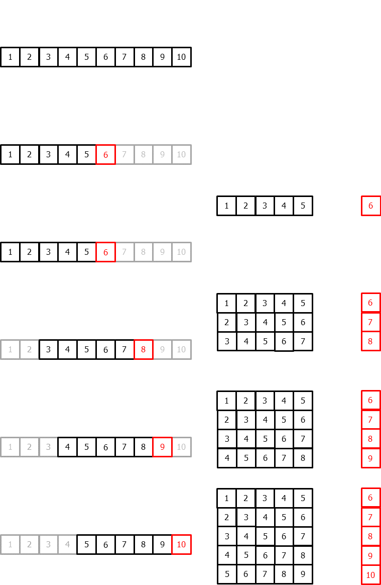
为了将机器学习模型应用于预测问题,需要把时间序列转换为一个矩阵,使得每个值都与其之前的时间窗口(滞后项,lags)相关联。
在时间序列的语境中,相对于时刻 $t$ 的滞后量(lag)被定义为序列在之前时刻的取值。例如,lag 1 是时刻 $t - 1$ 的值,而 lag $m$ 是时刻 $t - m$ 的值。
这种转换也允许加入额外的变量作为特征。
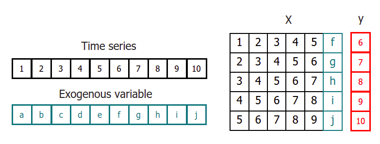
一旦将数据重排为上述形状,就可以训练任意回归模型来预测序列的下一个值(下一步)。在训练过程中,每一行都被视为一个独立样本,其中滞后 1、2、...、$p$ 的取值作为特征,用于预测时间步 $t + 1$ 的目标值。
多步时间序列预测
在时间序列任务中,很少只需要预测下一个值($t+1$)。更常见的目标是预测一个未来区间($t+1$, ..., $t+n$),或某个更远的时间点($t+n$)。为此可以采用多种策略来生成这种类型的预测。以下各节介绍 skforecast 中实现的主要策略。
递归式多步预测
由于预测 $t+n$ 需要用到 $t+n-1$ 时刻的值,而该值在预测时未知,因此采用递归式过程:每一个新预测都以前一个预测为基础。这一过程称为递归式预测(recursive forecasting)或递归式多步预测,可通过 ForecasterRecursive 类轻松实现。由于预测值会被用作后续步长的输入,误差可能沿预测区间逐步累积。


直接式多步预测
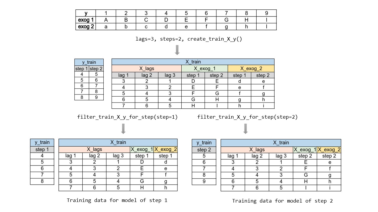
直接式多步预测(direct multi-step forecasting)为预测区间中的每一个步长训练一个独立模型。例如,要预测时间序列的未来 5 个取值,就要训练 5 个不同的模型,每个模型专注于其中一个步长。因此,不同步长上的预测彼此独立。


该方法的主要复杂性在于需要为每个步长生成正确的训练矩阵。skforecast 库中的 ForecasterDirect 类可将这一过程自动化。此外需要注意,此策略的计算成本更高,因为需要训练多个模型。下图展示了当响应变量与两个外生变量均可用时的处理流程。
多输出预测
某些机器学习模型(例如长短期记忆网络,LSTM)可以一次性(one-shot)同时预测序列的多个值。skforecast 库在 ForecasterRnn 类中实现了这种策略。
依赖库
本指南所用到的主要依赖如下:
# 数据处理
# ==============================================================================
import numpy as np
import pandas as pd
from skforecast.datasets import fetch_dataset
# 绘图
# ==============================================================================
import matplotlib.pyplot as plt
from skforecast.plot import set_dark_theme, plot_prediction_intervals
# 建模与预测
# ==============================================================================
import sklearn
from sklearn.linear_model import Ridge
from sklearn.ensemble import RandomForestRegressor
from sklearn.metrics import mean_squared_error, mean_absolute_error
from sklearn.preprocessing import StandardScaler
import skforecast
from skforecast.recursive import ForecasterRecursive
from skforecast.direct import ForecasterDirect
from skforecast.model_selection import (
TimeSeriesFold,
grid_search_forecaster,
backtesting_forecaster
)
from skforecast.preprocessing import RollingFeatures
from skforecast.utils import save_forecaster, load_forecaster
from skforecast.metrics import calculate_coverage
from skforecast.exceptions import LongTrainingWarning
import shap
# 警告配置
# ==============================================================================
import warnings
warnings.filterwarnings('once')
color = '\033[1m\033[38;5;208m'
print(f'{color}Version skforecast: {skforecast.__version__}')
print(f'{color}Version scikit-learn: {sklearn.__version__}')
print(f'{color}Version pandas: {pd.__version__}')
print(f'{color}Version numpy: {np.__version__}')
Version skforecast: 0.25.0 Version scikit-learn: 1.7.2 Version pandas: 2.3.3 Version numpy: 2.4.6
数据
本例提供了一条时间序列,表示 1992 至 2008 年间澳大利亚公共医疗系统在皮质类固醇药物上的每月支出(单位:百万美元)。我们的目标是创建一个自回归模型来预测未来的月度支出。本文所用数据来自经典教材 Forecasting: Principles and Practice by Rob J Hyndman and George Athanasopoulos。
# 数据下载
# ==============================================================================
data = fetch_dataset(name='h2o_exog', raw=True)
╭─────────────────────────────────── h2o_exog ────────────────────────────────────╮ │ Description: │ │ Monthly expenditure ($AUD) on corticosteroid drugs that the Australian health │ │ system had between 1991 and 2008. Two additional variables (exog_1, exog_2) are │ │ simulated. │ │ │ │ Source: │ │ Hyndman R (2023). fpp3: Data for Forecasting: Principles and Practice (3rd │ │ Edition). http://pkg.robjhyndman.com/fpp3package/, │ │ https://github.com/robjhyndman/fpp3package, http://OTexts.com/fpp3. │ │ │ │ URL: │ │ https://raw.githubusercontent.com/skforecast/skforecast- │ │ datasets/main/data/h2o_exog.csv │ │ │ │ Shape: 195 rows x 4 columns │ ╰─────────────────────────────────────────────────────────────────────────────────╯
原始数据集将日期存储在名为 fecha 的列中,首先将其重命名为 date。该列以 string 存储。使用 pd.to_datetime() 可将其转换为 datetime。转换后,将其设为索引以方便使用 Pandas 的时间序列功能。同时由于数据为按月记录,频率设置为 Month Start('MS')。
# 数据准备
# ==============================================================================
data = data.rename(columns={'fecha': 'date'})
data['date'] = pd.to_datetime(data['date'], format='%Y-%m-%d')
data = data.set_index('date')
data = data.sort_index()
data = data.asfreq('MS')
data.head()
| y | exog_1 | exog_2 | |
|---|---|---|---|
| date | |||
| 1992-04-01 | 0.379808 | 0.958792 | 1.166029 |
| 1992-05-01 | 0.361801 | 0.951993 | 1.117859 |
| 1992-06-01 | 0.410534 | 0.952955 | 1.067942 |
| 1992-07-01 | 0.483389 | 0.958078 | 1.097376 |
| 1992-08-01 | 0.475463 | 0.956370 | 1.122199 |
在 Pandas 中使用 asfreq() 方法时,会为匹配指定频率而自动用 NaN 填充时间序列中的缺口。因此,在该转换之后务必检查是否产生了缺失值。
# 缺失值
# ==============================================================================
print(f'Number of rows with missing values: {data.isnull().any(axis=1).sum()}')
Number of rows with missing values: 0
下面的检查用于确认日期索引是完整的、没有缺口。如果发现缺口,可以使用 asfreq() 进行填补,如下方被注释的代码行所示。
# 校验时间索引是否完整
# ==============================================================================
start_date = data.index.min()
end_date = data.index.max()
complete_date_range = pd.date_range(
start=start_date, end=end_date, freq=data.index.freq
)
is_index_complete = data.index.equals(complete_date_range)
print(f'Index complete: {is_index_complete}')
Index complete: True
# 在时间索引中填补缺口
# ==============================================================================
# 仅当索引不完整时才需要:缺失的日期会以 NaN 值补入
# data = data.asfreq(freq='MS', fill_value=np.nan)
使用最后 36 个月作为测试集以评估模型的预测能力。
# 训练集 / 测试集 划分
# ==============================================================================
steps = 36
data_train = data[:-steps]
data_test = data[-steps:]
print(
f'Train dates : {data_train.index.min()} --- '
f'{data_train.index.max()} (n={len(data_train)})'
)
print(
f'Test dates : {data_test.index.min()} --- '
f'{data_test.index.max()} (n={len(data_test)})'
)
set_dark_theme()
fig, ax = plt.subplots(figsize=(6, 2.5))
data_train['y'].plot(ax=ax, label='train')
data_test['y'].plot(ax=ax, label='test')
ax.legend();
Train dates : 1992-04-01 00:00:00 --- 2005-06-01 00:00:00 (n=159) Test dates : 2005-07-01 00:00:00 --- 2008-06-01 00:00:00 (n=36)

递归式多步预测
使用 ForecasterRecursive 类,基于 RandomForestRegressor 并设置 6 个滞后项作为时间窗口来创建并训练一个预测模型。这意味着模型使用过去 6 个月作为特征。这里以 6 个滞后项作为起点;最优的滞后项数量将在超参数调优阶段确定。
# 创建并训练预测器(forecaster)
# ==============================================================================
forecaster = ForecasterRecursive(
estimator = RandomForestRegressor(random_state=123),
lags = 6
)
forecaster.fit(y=data_train['y'])
forecaster
ForecasterRecursive
General Information
- Estimator: RandomForestRegressor
- Lags: [1 2 3 4 5 6]
- Window features: None
- Calendar features: None
- Window size: 6
- Series name: y
- Exogenous included: False
- Categorical features: auto
- Weight function included: False
- Differentiation order: None
- Drop NaN from series: False
- Creation date: 2026-09-22 09:16:52
- Last fit date: 2026-09-22 09:16:52
- Skforecast version: 0.25.0
- Python version: 3.13.14
- Forecaster id: None
Exogenous Variables
None
Data Transformations
- Transformer for y: None
- Transformer for exog: None
Training Information
- Training range: [Timestamp('1992-04-01 00:00:00'), Timestamp('2005-06-01 00:00:00')]
- Training index type: DatetimeIndex
- Training index frequency: MS
Estimator Parameters
-
{'bootstrap': True, 'ccp_alpha': 0.0, 'criterion': 'squared_error', 'max_depth': None, 'max_features': 1.0, 'max_leaf_nodes': None, 'max_samples': None, 'min_impurity_decrease': 0.0, 'min_samples_leaf': 1, 'min_samples_split': 2, 'min_weight_fraction_leaf': 0.0, 'monotonic_cst': None, 'n_estimators': 100, 'n_jobs': None, 'oob_score': False, 'random_state': 123, 'verbose': 0, 'warm_start': False}
Fit Kwargs
-
{}
预测
模型训练完成后,即可对测试集进行预测(向前 36 个月)。
# 预测
# ==============================================================================
predictions = forecaster.predict(steps=steps)
predictions.head()
2005-07-01 0.878756 2005-08-01 0.882167 2005-09-01 0.973184 2005-10-01 0.983678 2005-11-01 0.849494 Freq: MS, Name: pred, dtype: float64
# 绘制预测与测试集对比
# ==============================================================================
fig, ax = plt.subplots(figsize=(6, 2.5))
data_train['y'].plot(ax=ax, label='train')
data_test['y'].plot(ax=ax, label='test')
predictions.plot(ax=ax, label='predictions')
ax.legend();

测试集上的预测误差
为了量化模型预测误差,这里使用均方误差(MSE)度量。
# 测试误差
# ==============================================================================
error_mse = mean_squared_error(
y_true = data_test['y'],
y_pred = predictions
)
print(f'Test error (MSE): {error_mse}')
Test error (MSE): 0.0732683397612037
超参数调优
前述 ForecasterRecursive 使用 6 个滞后项作为特征,并采用默认超参数的 随机森林 回归器。然而,这些取值未必是最优的。Skforecast 提供了多种搜索策略用于选择最佳超参数与滞后项组合。本例使用 grid_search_forecaster,它会比较每个超参数与滞后项组合得到的结果,并找出最优配置。
💡 提示
超参数调优的计算成本高度依赖于用于评估每个组合的回测(backtesting)策略。通常,涉及的重训练(re-train)次数越多,调优耗时越长。
为了高效推进原型阶段,推荐采用两步法:首先在初筛时使用 refit=False 来快速缩小候选范围;随后聚焦于“感兴趣区域”,并根据具体业务需求配置合适的回测策略。更多回测策略建议参见 Hyperparameter tuning and lags selection。
# 超参数:网格搜索
# ==============================================================================
forecaster = ForecasterRecursive(
estimator = RandomForestRegressor(random_state=123),
lags = 12 # 此值将在网格搜索中被替换
)
# 训练与验证折
cv = TimeSeriesFold(
steps = 36,
initial_train_size = int(len(data_train) * 0.5),
fixed_train_size = False,
refit = False,
)
# 候选滞后项取值
lags_grid = [10, 20]
# 回归器超参数候选值
param_grid = {
'n_estimators': [100, 250],
'max_depth': [3, 8]
}
results_grid = grid_search_forecaster(
forecaster = forecaster,
y = data_train['y'],
cv = cv,
param_grid = param_grid,
lags_grid = lags_grid,
metric = 'mean_squared_error',
return_best = True,
n_jobs = 'auto',
verbose = False
)
# 搜索结果
# ==============================================================================
results_grid
| lags | lags_label | params | mean_squared_error | max_depth | n_estimators | |
|---|---|---|---|---|---|---|
| 0 | [1, 2, 3, 4, 5, 6, 7, 8, 9, 10, 11, 12, 13, 14... | [1, 2, 3, 4, 5, 6, 7, 8, 9, 10, 11, 12, 13, 14... | {'max_depth': 3, 'n_estimators': 250} | 0.021773 | 3 | 250 |
| 1 | [1, 2, 3, 4, 5, 6, 7, 8, 9, 10, 11, 12, 13, 14... | [1, 2, 3, 4, 5, 6, 7, 8, 9, 10, 11, 12, 13, 14... | {'max_depth': 8, 'n_estimators': 250} | 0.022068 | 8 | 250 |
| 2 | [1, 2, 3, 4, 5, 6, 7, 8, 9, 10, 11, 12, 13, 14... | [1, 2, 3, 4, 5, 6, 7, 8, 9, 10, 11, 12, 13, 14... | {'max_depth': 3, 'n_estimators': 100} | 0.022569 | 3 | 100 |
| 3 | [1, 2, 3, 4, 5, 6, 7, 8, 9, 10, 11, 12, 13, 14... | [1, 2, 3, 4, 5, 6, 7, 8, 9, 10, 11, 12, 13, 14... | {'max_depth': 8, 'n_estimators': 100} | 0.023562 | 8 | 100 |
| 4 | [1, 2, 3, 4, 5, 6, 7, 8, 9, 10] | [1, 2, 3, 4, 5, 6, 7, 8, 9, 10] | {'max_depth': 3, 'n_estimators': 100} | 0.063144 | 3 | 100 |
| 5 | [1, 2, 3, 4, 5, 6, 7, 8, 9, 10] | [1, 2, 3, 4, 5, 6, 7, 8, 9, 10] | {'max_depth': 3, 'n_estimators': 250} | 0.064241 | 3 | 250 |
| 6 | [1, 2, 3, 4, 5, 6, 7, 8, 9, 10] | [1, 2, 3, 4, 5, 6, 7, 8, 9, 10] | {'max_depth': 8, 'n_estimators': 250} | 0.064546 | 8 | 250 |
| 7 | [1, 2, 3, 4, 5, 6, 7, 8, 9, 10] | [1, 2, 3, 4, 5, 6, 7, 8, 9, 10] | {'max_depth': 8, 'n_estimators': 100} | 0.068730 | 8 | 100 |
最优结果对应于使用 20 个滞后项,以及随机森林超参数 {'max_depth': 3, 'n_estimators': 250} 的组合。
值得注意的是这一改进的来源。所有使用 20 个滞后项的配置误差都很接近(约 0.022),而所有使用 10 个滞后项的配置表现都明显更差(介于 0.063 与 0.069 之间),且与随机森林的超参数无关。因此,改进主要来自滞后项的数量:使用 20 个滞后项时,模型可以利用滞后 12,它刻画了序列的年度季节性。后文的模型可解释性一节也印证了这一点:lag_12 是最重要的特征,且远超其他特征。
最终模型
最后,使用找到的最优配置训练一个 ForecasterRecursive。由于在 grid_search_forecaster 中设置了 return_best=True,预测器已经按最优配置更新并重新训练,因此这一步并非必需,此处仅作演示之用。
# 使用最佳超参数与滞后项创建并训练预测器
# ==============================================================================
estimator = RandomForestRegressor(n_estimators=250, max_depth=3, random_state=123)
forecaster = ForecasterRecursive(
estimator = estimator,
lags = 20
)
forecaster.fit(y=data_train['y'])
# 预测
# ==============================================================================
predictions = forecaster.predict(steps=steps)
# 绘制预测与测试集对比
# ==============================================================================
fig, ax = plt.subplots(figsize=(6, 2.5))
data_train['y'].plot(ax=ax, label='train')
data_test['y'].plot(ax=ax, label='test')
predictions.plot(ax=ax, label='predictions')
ax.legend();

# 测试误差
# ==============================================================================
error_mse = mean_squared_error(
y_true = data_test['y'],
y_pred = predictions
)
print(f'Test error (MSE): {error_mse}')
Test error (MSE): 0.004356831371529948
最优的超参数与滞后项组合显著降低了测试误差,MSE 从 0.073 降至 0.0044。
回测(Backtesting)
为了获得模型预测能力的稳健估计,需要进行回测(backtesting)。回测是将预测模型回溯地应用于历史数据以评估其性能的一种方法,本质上是针对过去时段的特殊交叉验证。
✏️ 注意
为确保对模型进行准确评估,并对其在新数据上的预测性能建立信心,采用合适的回测策略至关重要。需要结合用例特征、可用计算资源以及预测间隔等因素来确定使用哪种策略。
一般而言,回测流程与真实上线场景越接近,得到的评估指标就越可靠。更多关于回测的信息,参见 Which strategy should I use?。
带重训练(refit)且训练集递增(固定起点,fixed origin)的回测
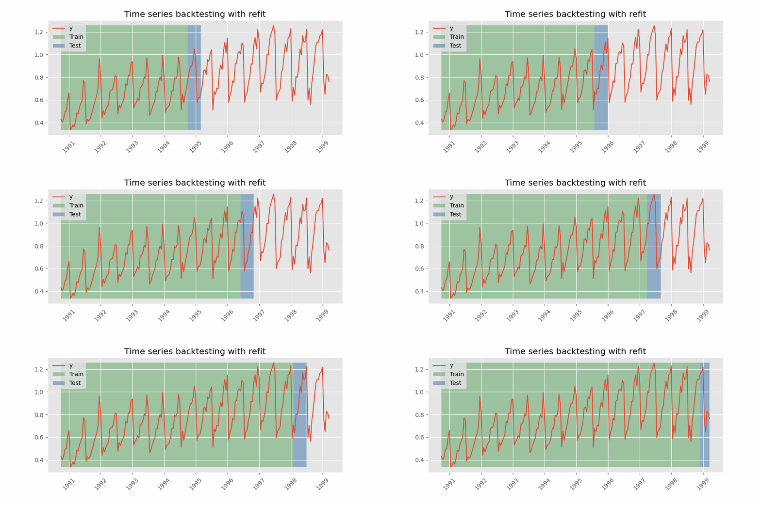
在每次预测之前都对模型进行训练。该设置使模型在每次迭代中都使用截至当时可用的全部数据。这是对标准交叉验证的一种变体:并非随机划分观测值,而是按时间顺序逐步增加训练集。
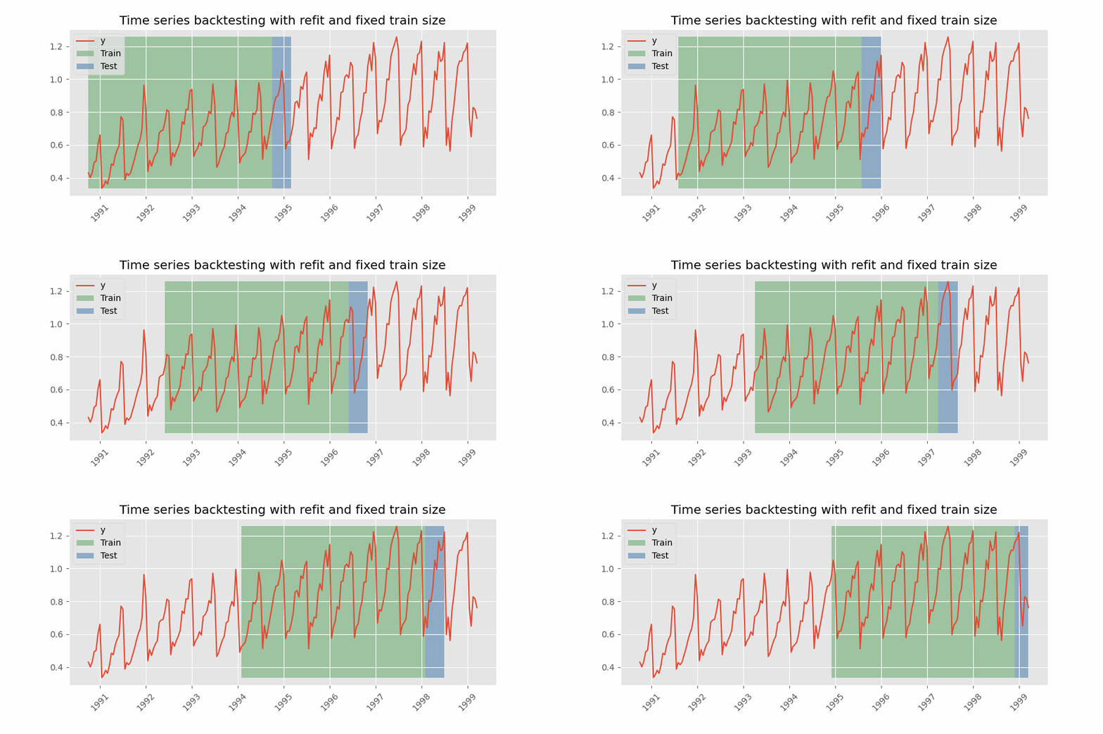
带重训练(refit)且固定训练集大小(滚动起点,rolling origin)的回测
与前者相似,但此处预测起点随时间向前滚动,因此训练集大小保持不变。这也常被称为时间序列交叉验证或逐步前向验证(walk-forward validation)。
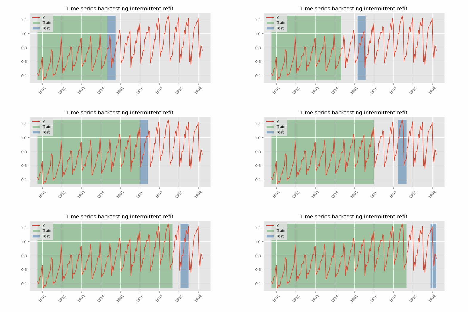
间歇性重训练(intermittent refit)的回测
模型每进行 $n$ 次预测迭代后再重训练一次。
💡 提示
该策略通常在重训练的计算成本与避免模型退化之间取得良好平衡。
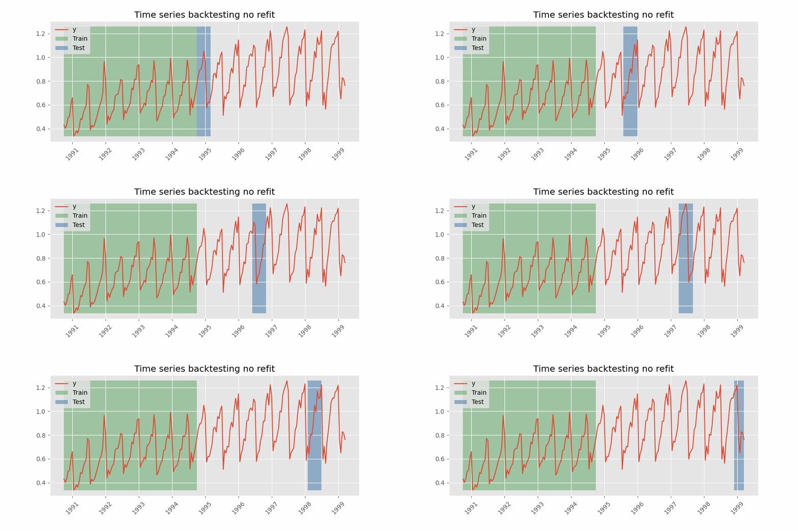
不重训练(no refit)的回测
完成一次初始训练后,模型按时间顺序顺序使用而不再更新。优势是只训练一次,速度更快;劣势是模型无法吸收最新数据,预测能力可能随时间减弱。
带步幅(stride)的回测
该方法用于控制相邻两个折之间测试集向前移动的距离。例如,你可能希望预测未来 30 天,但每 7 天生成一次新的预测。在这种设置下,每个测试窗口长 30 天(steps=30),而相邻折之间的步幅为一周(fold_stride=7)。这意味着各次预测会相互重叠,同一批观测会被预测多次,从而可以更全面地了解模型在不同预测起点下的一致性与稳定性。
根据 steps 与 fold_stride 的关系,输出结果可能包含重复的索引(当 fold_stride < steps 时)或出现间隔(当 fold_stride > steps 时)。
跳过折(Skip folds)
以上所有回测策略都可结合 skip_folds 参数跳过部分折次。由于模型在更少的时间点进行预测,计算成本降低、回测更快。这在只需粗略估计模型表现而非精确评估时尤其有用,例如超参数搜索。若 skip_folds 为整数,则返回每隔 skip_folds 个的折;若为列表,则跳过列表中指定的折。例如,若 skip_folds = 3 且共有 10 个折,则返回的折为 [0, 3, 6, 9];如果 skip_folds 为列表 [1, 2, 3],则返回的折为 [0, 4, 5, 6, 7, 8, 9]。
skforecast 库实现了多种回测策略。无论使用哪一种,都必须避免在搜索或优化过程中引入测试数据,否则会造成数据泄漏(data leakage),得到过于乐观的指标。
本例采用“带重训练且训练集递增(固定起点)”的回测策略。由于预测器的超参数和滞后项是使用 data_train 选定的,回测只在其后的时段(最后 36 个月)上进行,该时段未参与搜索。函数内部执行流程如下:
第一次迭代:使用选定的初始训练集(本例为 159 条观测,即
data_train的长度)训练模型,然后预测接下来的 12 条观测。第二次迭代:在初始训练集基础上再加入 12 条观测(159 + 12)后重新训练模型,然后预测接下来的 12 条观测。
重复上述过程直至用完所有可用观测。按照该策略,每次迭代训练集都会新增与预测步数相同数量的观测。
TimeSeriesFold 用于生成回测时训练/验证所需的分区。通过其多个参数可以灵活模拟诸如 refit、no refit、rolling origin 等场景。其 split 方法返回每个分区对应的时间序列索引位置;当设置 as_pandas=True 时,会返回包含详细信息与描述性列名的 DataFrame。
# 使用 TimeSeriesFold 生成回测分区
# ==============================================================================
cv = TimeSeriesFold(
steps = 12,
initial_train_size = len(data_train), # 网格搜索中使用的数据
window_size = 20,
fixed_train_size = False,
refit = True,
)
cv.split(X=data, as_pandas=True)
Information of folds
--------------------
Number of observations used for initial training: 159
Number of observations used for backtesting: 36
Number of folds: 3
Number skipped folds: 0
Number of steps per fold: 12
Number of steps to exclude between last observed data (last window) and predictions (gap): 0
Fold: 0
Training: 1992-04-01 00:00:00 -- 2005-06-01 00:00:00 (n=159)
Validation: 2005-07-01 00:00:00 -- 2006-06-01 00:00:00 (n=12)
Fold: 1
Training: 1992-04-01 00:00:00 -- 2006-06-01 00:00:00 (n=171)
Validation: 2006-07-01 00:00:00 -- 2007-06-01 00:00:00 (n=12)
Fold: 2
Training: 1992-04-01 00:00:00 -- 2007-06-01 00:00:00 (n=183)
Validation: 2007-07-01 00:00:00 -- 2008-06-01 00:00:00 (n=12)
| fold | train_start | train_end | last_window_start | last_window_end | test_start | test_end | test_start_with_gap | test_end_with_gap | fit_forecaster | |
|---|---|---|---|---|---|---|---|---|---|---|
| 0 | 0 | 0 | 159 | 139 | 159 | 159 | 171 | 159 | 171 | True |
| 1 | 1 | 0 | 171 | 151 | 171 | 171 | 183 | 171 | 183 | True |
| 2 | 2 | 0 | 183 | 163 | 183 | 183 | 195 | 183 | 195 | True |
与 backtesting_forecaster 联合使用时,无需显式指定 window_size,因为 backtesting_forecaster 会根据 forecaster 的配置自动确定该值,从而确保回测与模型需求完全对齐。
# 回测
# ==============================================================================
cv = TimeSeriesFold(
steps = 12,
initial_train_size = len(data_train),
fixed_train_size = False,
refit = True,
)
metric, predictions_backtest = backtesting_forecaster(
forecaster = forecaster,
y = data['y'],
cv = cv,
metric = 'mean_squared_error',
verbose = True
)
metric
Information of folds
--------------------
Number of observations used for initial training: 159
Number of observations used for backtesting: 36
Number of folds: 3
Number skipped folds: 0
Number of steps per fold: 12
Number of steps to exclude between last observed data (last window) and predictions (gap): 0
Fold: 0
Training: 1992-04-01 00:00:00 -- 2005-06-01 00:00:00 (n=159)
Validation: 2005-07-01 00:00:00 -- 2006-06-01 00:00:00 (n=12)
Fold: 1
Training: 1992-04-01 00:00:00 -- 2006-06-01 00:00:00 (n=171)
Validation: 2006-07-01 00:00:00 -- 2007-06-01 00:00:00 (n=12)
Fold: 2
Training: 1992-04-01 00:00:00 -- 2007-06-01 00:00:00 (n=183)
Validation: 2007-07-01 00:00:00 -- 2008-06-01 00:00:00 (n=12)
| mean_squared_error | |
|---|---|
| 0 | 0.005842 |
# 回测:预测 vs 真值
# ==============================================================================
fig, ax = plt.subplots(figsize=(6, 2.5))
data.loc[predictions_backtest.index, 'y'].plot(ax=ax, label='real values')
predictions_backtest['pred'].plot(ax=ax, label='predictions')
ax.legend();

回测得到的 MSE(0.0058)与之前在同一时段上得到的测试误差(0.0044)处于同一数量级。两个数值不必相同,因为它们回答的是不同的问题:测试误差衡量的是单个模型一次性预测 36 个月的表现,而回测衡量的是每次预测 12 个月、每年重新训练一次的模型的表现。一般而言,回测中使用的预测区间和重训练策略应与模型在生产环境中的使用方式一致,这样得到的指标才是对预期误差的可靠估计。
✏️ 注意
该预测器的超参数和滞后项仅使用 data_train(截至 2005-06 的数据)选定。因此,回测从 data_train 结束之后开始:用超参数搜索中已经使用过的观测来评估模型,会得到过于乐观的指标。
模型可解释性(特征重要性)
许多现代机器学习模型(如集成方法)具有高度复杂性,常被视为黑箱,难以解释其给出某个预测的原因。可解释性技术旨在揭示模型内部机理,帮助建立信任、提升透明度,并满足各领域的合规要求。增强模型可解释性不仅有助于理解模型行为,还能发现偏差、改进性能,并帮助利益相关者基于机器学习洞察做出更明智的决策。
Skforecast 兼容多种主流的模型可解释方法:模型特定的特征重要性、SHAP 值、以及部分依赖图(PDP)。
模型特定的特征重要性
# 提取特征重要性
# ==============================================================================
importance = forecaster.get_feature_importances()
importance.head(10)
| feature | importance | |
|---|---|---|
| 11 | lag_12 | 0.815564 |
| 1 | lag_2 | 0.086286 |
| 13 | lag_14 | 0.019047 |
| 9 | lag_10 | 0.013819 |
| 2 | lag_3 | 0.012943 |
| 14 | lag_15 | 0.009637 |
| 0 | lag_1 | 0.009141 |
| 10 | lag_11 | 0.008130 |
| 7 | lag_8 | 0.007377 |
| 8 | lag_9 | 0.005268 |
⚠️ 警告
仅当预测器(forecaster)内部的回归器具有 coef_ 或 feature_importances_ 属性时,get_feature_importances() 方法才会返回结果(scikit-learn 中大多数线性模型和基于树的模型都具备这些属性)。
SHAP 值
SHAP(SHapley Additive exPlanations)是一种流行的模型解释方法,可帮助从可视化与量化两方面理解变量及其取值对预测的影响。
在 skforecast 中,仅需以下两个要素即可生成 SHAP 解释:
预测器内部的回归器。
由时间序列构建并用于拟合预测器的训练矩阵。
基于这两部分,用户即可为 skforecast 模型创建具有洞察力、可解释的分析:用于验证模型可靠性、识别对预测影响最大的因素,并更深入地理解输入变量与目标之间的关系。
# 用于拟合内部回归器的训练矩阵
# ==============================================================================
X_train, y_train = forecaster.create_train_X_y(y=data_train['y'])
# 创建 SHAP 解释器(适用于树模型)
# ==============================================================================
explainer = shap.TreeExplainer(forecaster.estimator)
# 抽样 50% 数据以加速计算
rng = np.random.default_rng(seed=785412)
sample_idx = rng.choice(X_train.index, size=len(X_train)//2, replace=False)
X_train_sample = X_train.loc[sample_idx]
shap_values = explainer.shap_values(X_train_sample)
# SHAP 总结图(前 10 个特征)
# ==============================================================================
shap.summary_plot(shap_values, X_train_sample, max_display=10, show=False)
fig, ax = plt.gcf(), plt.gca()
ax.set_title('SHAP Summary plot')
ax.tick_params(labelsize=8, colors='white')
fig.set_size_inches(6, 3.5)

✏️ 注意
SHAP 库提供了多种解释器,分别适用于不同类型的模型。本例中使用的 shap.TreeExplainer 适用于树模型,例如 RandomForestRegressor。更多信息见 SHAP 文档。
单个预测的可解释性
SHAP 值不仅可以解释模型的整体行为,也是分析单个预测的有力工具。当需要理解某个具体预测是如何产生的、哪些变量对其有贡献时,这一点尤其有用。
要进行这种分析,需要获取预测时刻的特征取值(本例中为各滞后项)。可以通过 create_predict_X 方法,或在 backtesting_forecaster 函数中设置 return_predictors=True 来实现。
假设我们希望解释日期 2006-04-01(属于测试集)对应的预测。要使解释有效,被解释的模型必须与生成该预测的模型相同。因此,回测配置为 initial_train_size=len(data_train) 且 refit=False:预测器只训练一次,所用数据和 random_state 与创建 SHAP 解释器时所用的模型相同,然后对测试时段进行预测。
# 在测试集上回测,并返回用于预测的特征取值
# ==============================================================================
cv = TimeSeriesFold(
steps = 12 * 3,
initial_train_size = len(data_train),
refit = False,
)
_, predictions_backtest = backtesting_forecaster(
forecaster = forecaster,
y = data['y'],
cv = cv,
metric = 'mean_squared_error',
return_predictors = True,
)
将 return_predictors=True 设为真后,会返回一个 DataFrame,其中包含预测值('pred')、其所属分区('fold'),以及生成该预测所使用的各个滞后项的取值。
# 预测值与特征取值
# ==============================================================================
predictions_backtest.head()
| fold | pred | lag_1 | lag_2 | lag_3 | lag_4 | lag_5 | lag_6 | lag_7 | lag_8 | ... | lag_11 | lag_12 | lag_13 | lag_14 | lag_15 | lag_16 | lag_17 | lag_18 | lag_19 | lag_20 | |
|---|---|---|---|---|---|---|---|---|---|---|---|---|---|---|---|---|---|---|---|---|---|
| 2005-07-01 | 0 | 0.901160 | 0.842263 | 0.695248 | 0.670505 | 0.652590 | 0.597639 | 1.170690 | 1.257238 | 1.216037 | ... | 0.994864 | 1.001593 | 0.856803 | 0.795129 | 0.739986 | 0.749014 | 0.667989 | 1.130125 | 1.223235 | 1.050838 |
| 2005-08-01 | 0 | 0.943315 | 0.901160 | 0.842263 | 0.695248 | 0.670505 | 0.652590 | 0.597639 | 1.170690 | 1.257238 | ... | 1.134432 | 0.994864 | 1.001593 | 0.856803 | 0.795129 | 0.739986 | 0.749014 | 0.667989 | 1.130125 | 1.223235 |
| 2005-09-01 | 0 | 1.078241 | 0.943315 | 0.901160 | 0.842263 | 0.695248 | 0.670505 | 0.652590 | 0.597639 | 1.170690 | ... | 1.181011 | 1.134432 | 0.994864 | 1.001593 | 0.856803 | 0.795129 | 0.739986 | 0.749014 | 0.667989 | 1.130125 |
| 2005-10-01 | 0 | 1.107162 | 1.078241 | 0.943315 | 0.901160 | 0.842263 | 0.695248 | 0.670505 | 0.652590 | 0.597639 | ... | 1.216037 | 1.181011 | 1.134432 | 0.994864 | 1.001593 | 0.856803 | 0.795129 | 0.739986 | 0.749014 | 0.667989 |
| 2005-11-01 | 0 | 1.110907 | 1.107162 | 1.078241 | 0.943315 | 0.901160 | 0.842263 | 0.695248 | 0.670505 | 0.652590 | ... | 1.257238 | 1.216037 | 1.181011 | 1.134432 | 0.994864 | 1.001593 | 0.856803 | 0.795129 | 0.739986 | 0.749014 |
5 rows × 22 columns
# 针对单次预测的 SHAP 瀑布图
# ==============================================================================
predictors = predictions_backtest.drop(columns=['pred', 'fold'])
shap_values_single = explainer(predictors.loc[['2006-04-01']])
shap.plots.waterfall(shap_values_single[0], show=False)
fig, ax = plt.gcf(), plt.gca()
fig.set_size_inches(6, 3.5)
plt.show()

在该日期上,预测值(0.714)低于模型的平均预测值($E[f(X)]$ = 0.779)。影响最大的特征是 lag_12:序列在 12 个月前的取值(0.671)相对较低,使预测值降低了 0.08。其余滞后项的影响要小得多,其中 lag_2 为负向贡献,lag_10 为正向贡献。图中显示的 $f(x)$ 与该日期的预测值一致,这证实了被解释的模型正是生成该预测的模型。
含外生变量的预测
在前面的示例中,仅使用被预测变量自身的滞后项作为特征。在某些场景中,可以获得其他变量的信息,且这些变量的未来取值是已知的,因此可以作为额外特征加入模型。
沿用上一示例,数据集中包含一个模拟变量 exog_1,其行为与目标时间序列相关,因此将其作为特征纳入。
✏️ 注意
自 0.22.0 版本起,可以使用 categorical_features 参数,方便地将类别变量作为特征纳入预测模型。更多信息参见 skforecast 文档。在本例中不需要该参数,因为外生变量 exog_1 是数值型的。
# 绘制目标变量与外生变量
# ==============================================================================
fig, ax = plt.subplots(figsize=(6, 2.7))
data['y'].plot(ax=ax, label='y')
data['exog_1'].plot(ax=ax, label='exogenous variable')
ax.legend(loc='upper left')
plt.show()

# 训练集 / 测试集 划分
# ==============================================================================
steps = 36
data_train = data[:-steps]
data_test = data[-steps:]
print(
f'Train dates : {data_train.index.min()} --- '
f'{data_train.index.max()} (n={len(data_train)})'
)
print(
f'Test dates : {data_test.index.min()} --- '
f'{data_test.index.max()} (n={len(data_test)})'
)
Train dates : 1992-04-01 00:00:00 --- 2005-06-01 00:00:00 (n=159) Test dates : 2005-07-01 00:00:00 --- 2008-06-01 00:00:00 (n=36)
# 创建并训练预测器(含外生变量)
# ==============================================================================
forecaster = ForecasterRecursive(
estimator = RandomForestRegressor(random_state=123),
lags = 8
)
forecaster.fit(y=data_train['y'], exog=data_train['exog_1'])
由于 ForecasterRecursive 在训练时包含了外生变量,调用 predict() 进行预测时必须同时传入该变量的未来取值。
⚠️ 警告
外生变量的未来取值必须在预测时可用。如果这些取值无法提前获知而需要自行预测,其误差会传播到目标序列的预测中。同样,如果评估模型时使用了在生产环境中无法获知的外生变量真实值,得到的指标会过于乐观。
# 预测
# ==============================================================================
predictions = forecaster.predict(steps=steps, exog=data_test['exog_1'])
# 绘图
# ==============================================================================
fig, ax = plt.subplots(figsize=(6, 2.5))
data_train['y'].plot(ax=ax, label='train')
data_test['y'].plot(ax=ax, label='test')
predictions.plot(ax=ax, label='predictions')
ax.legend()
plt.show()

# 测试误差
# ==============================================================================
error_mse = mean_squared_error(
y_true = data_test['y'],
y_pred = predictions
)
print(f'Test error (MSE): {error_mse}')
Test error (MSE): 0.03989087922533574
测试误差(MSE 为 0.040)低于不含外生变量的初始模型(0.073)。不过,这一比较仅供参考,因为两个模型使用的滞后项数量不同(8 与 6),且都未经过调优。
窗口与自定义特征
在时间序列预测中,除了滞后项之外,考虑额外的统计特征也常常有用。例如,前 n 个值的移动平均可以帮助捕捉趋势。通过参数 window_features,可以纳入由过去取值计算得到的额外特征。
skforecast 提供的 RollingFeatures(滑动窗口特征)类支持创建一些最常用的特征:
- 'mean':前 n 个值的平均值。
- 'std':前 n 个值的标准差。
- 'min':前 n 个值的最小值。
- 'max':前 n 个值的最大值。
- 'sum':前 n 个值的求和。
- 'median':前 n 个值的中位数。
- 'ratio_min_max':前 n 个值最小值与最大值之比。
- 'coef_variation':前 n 个值的变异系数。
可以为每种统计指定不同的窗口大小,也可以统一设置同一窗口大小。
⚠️ 警告
RollingFeatures 非常适合用来引入一些最常用的特征。不过,用户可能需要使用该类未提供的其他特征。此时,用户可以自行创建一个类来计算所需特征,并将其传入预测器。更多信息参见 window-features 文档。
# 训练集 / 测试集 划分
# ==============================================================================
steps = 36
data_train = data[:-steps]
data_test = data[-steps:]
print(
f'Train dates : {data_train.index.min()} --- '
f'{data_train.index.max()} (n={len(data_train)})'
)
print(
f'Test dates : {data_test.index.min()} --- '
f'{data_test.index.max()} (n={len(data_test)})'
)
Train dates : 1992-04-01 00:00:00 --- 2005-06-01 00:00:00 (n=159) Test dates : 2005-07-01 00:00:00 --- 2008-06-01 00:00:00 (n=36)
创建并训练一个新的 ForecasterRecursive(使用 RandomForestRegressor),除 10 个滞后项外,同时加入最近 20 个值的移动平均、最大值、最小值与标准差等窗口特征。
# 窗口特征
# ==============================================================================
window_features = RollingFeatures(
stats = ['mean', 'std', 'min', 'max'],
window_sizes = 20
)
# 创建并训练预测器
# ==============================================================================
forecaster = ForecasterRecursive(
estimator = RandomForestRegressor(random_state=123),
lags = 10,
window_features = window_features,
)
forecaster.fit(y=data_train['y'])
forecaster
ForecasterRecursive
General Information
- Estimator: RandomForestRegressor
- Lags: [ 1 2 3 4 5 6 7 8 9 10]
- Window features: ['roll_mean_20', 'roll_std_20', 'roll_min_20', 'roll_max_20']
- Calendar features: None
- Window size: 20
- Series name: y
- Exogenous included: False
- Categorical features: auto
- Weight function included: False
- Differentiation order: None
- Drop NaN from series: False
- Creation date: 2026-09-22 09:17:17
- Last fit date: 2026-09-22 09:17:17
- Skforecast version: 0.25.0
- Python version: 3.13.14
- Forecaster id: None
Exogenous Variables
None
Data Transformations
- Transformer for y: None
- Transformer for exog: None
Training Information
- Training range: [Timestamp('1992-04-01 00:00:00'), Timestamp('2005-06-01 00:00:00')]
- Training index type: DatetimeIndex
- Training index frequency: MS
Estimator Parameters
-
{'bootstrap': True, 'ccp_alpha': 0.0, 'criterion': 'squared_error', 'max_depth': None, 'max_features': 1.0, 'max_leaf_nodes': None, 'max_samples': None, 'min_impurity_decrease': 0.0, 'min_samples_leaf': 1, 'min_samples_split': 2, 'min_weight_fraction_leaf': 0.0, 'monotonic_cst': None, 'n_estimators': 100, 'n_jobs': None, 'oob_score': False, 'random_state': 123, 'verbose': 0, 'warm_start': False}
Fit Kwargs
-
{}
create_train_X_y 方法可访问在预测器训练过程中内部生成并用于拟合模型的训练矩阵。这样用户可以检查数据并理解这些特征是如何创建的。注意,训练矩阵的第一个日期是 1993-12-01,而不是 1992-04-01:前 20 条观测无法作为训练目标,因为最大的窗口(20)需要同样数量的历史值才能计算。
# 训练矩阵
# ==============================================================================
X_train, y_train = forecaster.create_train_X_y(y=data_train['y'])
display(X_train.head())
display(y_train.head())
| lag_1 | lag_2 | lag_3 | lag_4 | lag_5 | lag_6 | lag_7 | lag_8 | lag_9 | lag_10 | roll_mean_20 | roll_std_20 | roll_min_20 | roll_max_20 | |
|---|---|---|---|---|---|---|---|---|---|---|---|---|---|---|
| date | ||||||||||||||
| 1993-12-01 | 0.699605 | 0.632947 | 0.601514 | 0.558443 | 0.509210 | 0.470126 | 0.428859 | 0.413890 | 0.427283 | 0.387554 | 0.523089 | 0.122733 | 0.361801 | 0.771258 |
| 1994-01-01 | 0.963081 | 0.699605 | 0.632947 | 0.601514 | 0.558443 | 0.509210 | 0.470126 | 0.428859 | 0.413890 | 0.427283 | 0.552253 | 0.152567 | 0.361801 | 0.963081 |
| 1994-02-01 | 0.819325 | 0.963081 | 0.699605 | 0.632947 | 0.601514 | 0.558443 | 0.509210 | 0.470126 | 0.428859 | 0.413890 | 0.575129 | 0.156751 | 0.387554 | 0.963081 |
| 1994-03-01 | 0.437670 | 0.819325 | 0.963081 | 0.699605 | 0.632947 | 0.601514 | 0.558443 | 0.509210 | 0.470126 | 0.428859 | 0.576486 | 0.155363 | 0.387554 | 0.963081 |
| 1994-04-01 | 0.506121 | 0.437670 | 0.819325 | 0.963081 | 0.699605 | 0.632947 | 0.601514 | 0.558443 | 0.509210 | 0.470126 | 0.577622 | 0.154728 | 0.387554 | 0.963081 |
date 1993-12-01 0.963081 1994-01-01 0.819325 1994-02-01 0.437670 1994-03-01 0.506121 1994-04-01 0.470491 Freq: MS, Name: y, dtype: float64
# 预测
# ==============================================================================
predictions = forecaster.predict(steps=steps)
# 绘图
# ==============================================================================
fig, ax = plt.subplots(figsize=(6, 2.5))
data_train['y'].plot(ax=ax, label='train')
data_test['y'].plot(ax=ax, label='test')
predictions.plot(ax=ax, label='predictions')
ax.legend()
plt.show()

# 测试误差
# ==============================================================================
error_mse = mean_squared_error(
y_true = data_test['y'],
y_pred = predictions
)
print(f'Test error (MSE): {error_mse}')
Test error (MSE): 0.041801435904318146
在本例中,测试误差(MSE 为 0.042)远高于使用 20 个滞后项的调优模型(0.0044)。最相关的信息,即序列在 12 个月前的取值,在只有 10 个滞后项时无法获得,而滚动统计量并不能替代它。与滞后项和超参数一样,窗口特征的选择也应经过验证,例如通过回测。
直接式多步预测
ForecasterRecursive 采用递归式预测策略,即每一步预测依赖前一步预测。另一种做法是为每个待预测步长分别训练一个模型,即“直接式多步预测”。该策略因需训练多个模型而计算成本更高,但在某些场景下表现更好。可使用 ForecasterDirect 类构建此类模型,并可包含一个或多个外生变量。
⚠️ 警告
ForecasterDirect 可能需要较长的训练时间,因为它会为每一个步长各自拟合一个模型。
与 ForecasterRecursive 不同,ForecasterDirect 在创建时必须指定要预测的 steps 数,这意味着在执行 predict() 时无法超出最初定义的步数。
本例使用带 Ridge 正则化的线性模型(Ridge)作为回归器。带正则化的线性模型需要对特征进行标准化。由于滞后项由序列自身生成,通过 transformer_y 参数(本例为 StandardScaler)对序列进行缩放,也就同时标准化了这些特征。该变换在内部自动完成,预测结果会以原始尺度返回。
更多关于在 scikit-learn 中使用 transformer 与 pipeline 的文档,参见:skforecast with scikit-learn and transformers pipelines。
# 创建预测器
# ==============================================================================
forecaster = ForecasterDirect(
estimator = Ridge(),
steps = 36,
lags = 8, # 该值会在网格搜索中被替换
transformer_y = StandardScaler()
)
# 超参数网格搜索
# ==============================================================================
warnings.simplefilter('ignore', category=LongTrainingWarning)
cv = TimeSeriesFold(
steps = 36,
initial_train_size = int(len(data_train) * 0.5),
fixed_train_size = False,
refit = False,
)
param_grid = {'alpha': np.logspace(-5, 5, 10)}
lags_grid = [5, 12, 20]
results_grid = grid_search_forecaster(
forecaster = forecaster,
y = data_train['y'],
cv = cv,
param_grid = param_grid,
lags_grid = lags_grid,
metric = 'mean_squared_error',
return_best = True
)
# 搜索结果
# ==============================================================================
results_grid.head()
| lags | lags_label | params | mean_squared_error | alpha | |
|---|---|---|---|---|---|
| 0 | [1, 2, 3, 4, 5, 6, 7, 8, 9, 10, 11, 12] | [1, 2, 3, 4, 5, 6, 7, 8, 9, 10, 11, 12] | {'alpha': 0.2782559402207126} | 0.027414 | 0.278256 |
| 1 | [1, 2, 3, 4, 5, 6, 7, 8, 9, 10, 11, 12] | [1, 2, 3, 4, 5, 6, 7, 8, 9, 10, 11, 12] | {'alpha': 3.593813663804626} | 0.027435 | 3.593814 |
| 2 | [1, 2, 3, 4, 5, 6, 7, 8, 9, 10, 11, 12] | [1, 2, 3, 4, 5, 6, 7, 8, 9, 10, 11, 12] | {'alpha': 0.021544346900318846} | 0.027484 | 0.021544 |
| 3 | [1, 2, 3, 4, 5, 6, 7, 8, 9, 10, 11, 12] | [1, 2, 3, 4, 5, 6, 7, 8, 9, 10, 11, 12] | {'alpha': 0.0016681005372000592} | 0.027490 | 0.001668 |
| 4 | [1, 2, 3, 4, 5, 6, 7, 8, 9, 10, 11, 12] | [1, 2, 3, 4, 5, 6, 7, 8, 9, 10, 11, 12] | {'alpha': 0.0001291549665014884} | 0.027491 | 0.000129 |
最优结果为:使用 12 个滞后项,且 Ridge 的设置为 {'alpha': 0.278}。
# 预测
# ==============================================================================
predictions = forecaster.predict()
# 绘制预测与测试集对比
# ==============================================================================
fig, ax = plt.subplots(figsize=(6, 2.5))
data_train['y'].plot(ax=ax, label='train')
data_test['y'].plot(ax=ax, label='test')
predictions.plot(ax=ax, label='predictions')
ax.legend()
plt.show()

# 测试误差
# ==============================================================================
error_mse = mean_squared_error(
y_true = data_test['y'],
y_pred = predictions
)
print(f'Test error (MSE): {error_mse}')
Test error (MSE): 0.011792965469623131
测试误差(MSE 为 0.0118)高于调优后的递归式随机森林(0.0044)。这一差异不能仅归因于预测策略,因为回归器也不同(Ridge 与随机森林)。要公平地比较递归式与直接式策略,应使用相同的回归器和相同的验证流程。
概率预测
与点预测不同,概率预测是一类方法族,它预测的是结果的期望分布而非单一的未来值。概率预测提供了更丰富的信息,因为它可以构建预测区间,即真实值可能落入的范围。形式化地说,预测区间指在给定概率下,响应变量的真实值预计会出现的区间。
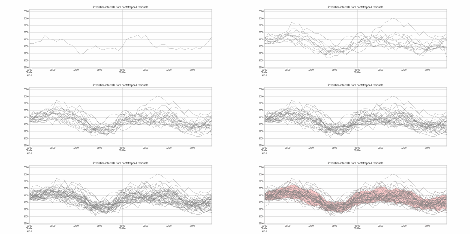
Skforecast 实现了多种概率预测方法:
# 训练集 / 测试集 划分
# ==============================================================================
steps = 36
data_train = data[:-steps]
data_test = data[-steps:]
print(
f'Train dates : {data_train.index.min()} --- '
f'{data_train.index.max()} (n={len(data_train)})'
)
print(
f'Test dates : {data_test.index.min()} --- '
f'{data_test.index.max()} (n={len(data_test)})'
)
Train dates : 1992-04-01 00:00:00 --- 2005-06-01 00:00:00 (n=159) Test dates : 2005-07-01 00:00:00 --- 2008-06-01 00:00:00 (n=36)
# 创建并训练预测器
# ==============================================================================
forecaster = ForecasterRecursive(
estimator = Ridge(alpha=0.1),
lags = 15
)
forecaster.fit(y=data_train['y'], store_in_sample_residuals=True)
# 预测区间
# ==============================================================================
predictions = forecaster.predict_interval(
steps = steps,
interval = [0.05, 0.95],
method = 'bootstrapping',
n_boot = 150
)
predictions.head()
| pred | lower_bound | upper_bound | |
|---|---|---|---|
| 2005-07-01 | 0.970598 | 0.788690 | 1.059012 |
| 2005-08-01 | 0.990932 | 0.815214 | 1.102761 |
| 2005-09-01 | 1.149609 | 1.064396 | 1.258934 |
| 2005-10-01 | 1.194584 | 1.098682 | 1.313509 |
| 2005-11-01 | 1.231744 | 1.122570 | 1.355601 |
# 预测误差
# ==============================================================================
error_mse = mean_squared_error(
y_true = data_test['y'],
y_pred = predictions['pred']
)
print(f'Test error (MSE): {error_mse}')
# 绘制带预测区间的预测结果
# ==============================================================================
fig, ax = plt.subplots(figsize=(6, 2.5))
plot_prediction_intervals(
predictions = predictions,
y_true = data_test,
target_variable = 'y',
ax = ax,
kwargs_fill_between = {'color': 'gray', 'alpha': 0.3, 'zorder': 1}
)
plt.show()
Test error (MSE): 0.010465086161791145

# 带预测区间的回测
# ==============================================================================
forecaster = ForecasterRecursive(
estimator = Ridge(alpha=0.1),
lags = 15
)
cv = TimeSeriesFold(
steps = 36,
initial_train_size = len(data) - 12 * 9,
fixed_train_size = False,
refit = True,
)
metric, predictions = backtesting_forecaster(
forecaster = forecaster,
y = data['y'],
cv = cv,
metric = 'mean_squared_error',
interval = [0.05, 0.95],
interval_method = 'bootstrapping',
n_boot = 150,
verbose = True
)
display(metric)
# 绘图
# ==============================================================================
fig, ax = plt.subplots(figsize=(6, 2.5))
plot_prediction_intervals(
predictions = predictions,
y_true = data.loc[predictions.index, :],
target_variable = 'y',
ax = ax,
kwargs_fill_between = {'color': 'gray', 'alpha': 0.3, 'zorder': 1}
)
plt.show()
Information of folds
--------------------
Number of observations used for initial training: 87
Number of observations used for backtesting: 108
Number of folds: 3
Number skipped folds: 0
Number of steps per fold: 36
Number of steps to exclude between last observed data (last window) and predictions (gap): 0
Fold: 0
Training: 1992-04-01 00:00:00 -- 1999-06-01 00:00:00 (n=87)
Validation: 1999-07-01 00:00:00 -- 2002-06-01 00:00:00 (n=36)
Fold: 1
Training: 1992-04-01 00:00:00 -- 2002-06-01 00:00:00 (n=123)
Validation: 2002-07-01 00:00:00 -- 2005-06-01 00:00:00 (n=36)
Fold: 2
Training: 1992-04-01 00:00:00 -- 2005-06-01 00:00:00 (n=159)
Validation: 2005-07-01 00:00:00 -- 2008-06-01 00:00:00 (n=36)
| mean_squared_error | |
|---|---|
| 0 | 0.012641 |

# 预测区间覆盖率(coverage)
# ==============================================================================
coverage = calculate_coverage(
y_true = data.loc[predictions.index, 'y'],
lower_bound = predictions['lower_bound'],
upper_bound = predictions['upper_bound'],
)
print(f'Predicted interval coverage: {round(100 * coverage, 2)} %')
Predicted interval coverage: 77.78 %
分位数 [0.05, 0.95] 定义了一个名义覆盖率为 90% 的区间,即预期有 90% 的真实值落在区间内。回测得到的经验覆盖率为 77.78%,明显低于名义值:区间过窄(过度自信)。当区间由样本内(in-sample)残差估计时,这种情况很常见,因为模型在自身训练数据上的误差往往小于在新数据上的误差。使用样本外(out-of-sample)残差,或用保序(conformal)方法校准区间,通常能使覆盖率更接近名义值。参见自助法残差与保序预测。
✏️ 注意
关于概率预测的更多信息,参见 Probabilistic forecasting with skforecast。
自定义评估指标
在回测(backtesting_forecaster)与超参数优化(grid_search_forecaster)过程中,除了常用的 mean_squared_error、mean_absolute_error 等指标外,也可以使用任意自定义函数,只要满足:
必须包含参数:
y_true:真实值。y_pred:预测值。
必须返回数值(
float或int)。指标应随模型改进而降低(即数值越低表示性能越好)。这一约束仅在
grid_search_forecaster中设置return_best=True时适用,因为 skforecast 会选择指标值最低的配置。
这使得模型可在多种场景下得到有针对性的评估,例如:
仅考虑某些月份、日期、小时……
仅考虑节假日的日期。
仅考虑预测视窗中的最后一步。
下面的示例展示了如何运行一个预测区间为 36 个月的回测,并在计算指标时仅考虑每年的最后 3 个月。这里复用了上一节中定义的预测器和 cv 对象。
# 自定义指标
# ==============================================================================
def custom_metric(y_true, y_pred):
"""
仅使用每年最后 3 个月的预测值来计算平均绝对误差。
"""
mask = y_true.index.month.isin([10, 11, 12])
mae = mean_absolute_error(y_true[mask], y_pred[mask])
return mae
# 回测
# ==============================================================================
metric, predictions_backtest = backtesting_forecaster(
forecaster = forecaster,
y = data['y'],
cv = cv,
metric = custom_metric,
verbose = True
)
metric
Information of folds
--------------------
Number of observations used for initial training: 87
Number of observations used for backtesting: 108
Number of folds: 3
Number skipped folds: 0
Number of steps per fold: 36
Number of steps to exclude between last observed data (last window) and predictions (gap): 0
Fold: 0
Training: 1992-04-01 00:00:00 -- 1999-06-01 00:00:00 (n=87)
Validation: 1999-07-01 00:00:00 -- 2002-06-01 00:00:00 (n=36)
Fold: 1
Training: 1992-04-01 00:00:00 -- 2002-06-01 00:00:00 (n=123)
Validation: 2002-07-01 00:00:00 -- 2005-06-01 00:00:00 (n=36)
Fold: 2
Training: 1992-04-01 00:00:00 -- 2005-06-01 00:00:00 (n=159)
Validation: 2005-07-01 00:00:00 -- 2008-06-01 00:00:00 (n=36)
| custom_metric | |
|---|---|
| 0 | 0.128159 |
保存与加载模型
可以使用 pickle 或 joblib 将 skforecast 模型保存/加载。为简化流程,提供了两个便捷函数:save_forecaster 与 load_forecaster,示例如下。更详细的文档参见:skforecast save and load forecaster。
# 创建预测器
# ==============================================================================
forecaster = ForecasterRecursive(
estimator = RandomForestRegressor(random_state=123),
lags = 3
)
forecaster.fit(y=data['y'])
forecaster.predict(steps=3)
2008-07-01 0.751967 2008-08-01 0.826505 2008-09-01 0.879444 Freq: MS, Name: pred, dtype: float64
# 保存预测器
# ==============================================================================
save_forecaster(forecaster, file_name='forecaster.joblib', verbose=False)
# 加载预测器
# ==============================================================================
forecaster_loaded = load_forecaster('forecaster.joblib')
===================
ForecasterRecursive
===================
Estimator: RandomForestRegressor
Lags: [1 2 3]
Window features: None
Calendar features: None
Window size: 3
Series name: y
Exogenous included: False
Exogenous names: None
Categorical features: auto
Transformer for y: None
Transformer for exog: None
Weight function included: False
Differentiation order: None
Drop NaN from series: False
Training range: [Timestamp('1992-04-01 00:00:00'), Timestamp('2008-06-01 00:00:00')]
Training index type: DatetimeIndex
Training index frequency: <MonthBegin>
Estimator parameters:
{'bootstrap': True, 'ccp_alpha': 0.0, 'criterion': 'squared_error', 'max_depth':
None, 'max_features': 1.0, 'max_leaf_nodes': None, 'max_samples': None,
'min_impurity_decrease': 0.0, 'min_samples_leaf': 1, 'min_samples_split': 2,
'min_weight_fraction_leaf': 0.0, 'monotonic_cst': None, 'n_estimators': 100,
'n_jobs': None, 'oob_score': False, 'random_state': 123, 'verbose': 0,
'warm_start': False}
fit_kwargs: {}
Creation date: 2026-09-22 09:17:21
Last fit date: 2026-09-22 09:17:21
Skforecast version: 0.25.0
Python version: 3.13.14
Forecaster id: None
# 预测
# ==============================================================================
forecaster_loaded.predict(steps=3)
2008-07-01 0.751967 2008-08-01 0.826505 2008-09-01 0.879444 Freq: MS, Name: pred, dtype: float64
⚠️ 警告
当预测器使用了自定义的窗口特征类或自定义的权重函数(weight_func)时,需要在加载预测器之前定义这些对象,否则会报错。因此,建议将它们保存在独立文件中,并在加载预测器之前先导入。
在生产环境中使用预测器
在预测相关项目中,通常会在实验与开发阶段之后产出一个模型。要使该模型对业务产生正向影响,必须能够将其投入生产,并定期生成预测以支持决策。
假设需要每周(例如每周一)生成预测。默认情况下,对训练好的预测器对象调用 predict 方法时,预测从最后一条训练观测之后开始。因此,可以每周在需要首次预测之前重新训练模型,然后调用其 predict 方法。
该策略简单直观,但有时并不可行,原因包括:
训练成本过高,无法频繁执行。
训练所用的历史数据不再可用。
预测频率过高,预测之间没有足够时间进行训练。
在这些场景中,即使近期未重训练,模型也必须能够随时进行预测。
所有使用 skforecast 训练生成的模型,其 predict 方法都带有 last_window 参数。通过该参数,可以仅提供生成自回归特征(滞后项)所需的最近历史值,从而在无需重训练的情况下完成预测。
更多文档参见:skforecast forecaster in production。
# 创建并训练预测器
# ==============================================================================
forecaster = ForecasterRecursive(
estimator = RandomForestRegressor(random_state=123),
lags = 6
)
forecaster.fit(y=data_train['y'])
由于模型使用最近 6 个滞后项作为特征,last_window 至少需要包含开始预测点之前的 6 个历史取值。
# 使用 last_window 进行预测
# ==============================================================================
last_window = data_test['y'][-6:]
forecaster.predict(last_window=last_window, steps=4)
2008-07-01 0.757750 2008-08-01 0.836313 2008-09-01 0.877668 2008-10-01 0.911734 Freq: MS, Name: pred, dtype: float64
如果预测器包含外生变量,除了 last_window 外,exog 参数还必须包含外生变量的未来取值。
其他功能
skforecast 的功能远不止本文所示,建议读者参考以下链接进一步了解该库:
示例与教程
我们也建议你探索我们的示例与教程合集,你将在其中找到大量用例,帮助你更直观地理解如何使用这一强大的库。
会话信息
import session_info
session_info.show(html=False)
----- matplotlib 3.10.9 numpy 2.4.6 pandas 2.3.3 session_info v1.0.1 shap 0.52.0 skforecast 0.25.0 sklearn 1.7.2 ----- IPython 9.15.0 jupyter_client 8.9.1 jupyter_core 5.9.1 ----- Python 3.13.14 | packaged by conda-forge | (main, Jun 12 2026, 09:44:26) [MSC v.1944 64 bit (AMD64)] Windows-11-10.0.26200-SP0 ----- Session information updated at 2026-09-22 09:17
🚀 推荐课程
如果你想更深入地学习时间序列预测的实战方法,我们强烈推荐 Train in Data 的 Forecasting with Machine Learning Course。作为我们社区的成员,通过此链接报名即可自动享受 10% 的折扣。
透明度声明:我们推荐该课程,是因为其技术严谨,且与我们的编辑方针高度契合。如果你决定报名,将直接支持 cienciadedatos.net 免费内容的维护与创作,而你无需支付任何额外费用。
参考文献
Hyndman, R.J., & Athanasopoulos, G. (2021) Forecasting: principles and practice, 第三版,OTexts:墨尔本,澳大利亚。
Svetunkov, I. (2023). Forecasting and Analytics with the Augmented Dynamic Adaptive Model (ADAM). Chapman and Hall/CRC.
Joseph, M. (2022). Modern time series forecasting with Python: Explore industry-ready time series forecasting using modern machine learning and Deep Learning. Packt 出版社。
Hilpisch, Y. (2018). Python for Finance: Mastering Data-Driven Finance (2nd ed.). O'Reilly Media.
引用
如何引用本文档
如果你在工作中使用了本文档或其中任何部分,请注明来源,谢谢!
Skforecast:使用Python和机器学习进行时间序列预测,作者 Joaquín Amat Rodrigo 与 Javier Escobar Ortiz,使用许可:Attribution-NonCommercial-ShareAlike 4.0 International (CC BY-NC-SA 4.0 DEED),网址:https://cienciadedatos.net/documentos/py27-time-series-forecasting-python-scikitlearn-cn.html
如何引用 skforecast
如果你在发表作品中使用了 skforecast,我们将非常感谢你引用已发布的软件。
Zenodo:
Amat Rodrigo, Joaquin, & Escobar Ortiz, Javier. (2026). skforecast (v0.25.0). Zenodo. https://doi.org/10.5281/zenodo.8382788
APA:
Amat Rodrigo, J., & Escobar Ortiz, J. (2026). skforecast (Version 0.25.0) [Computer software]. https://doi.org/10.5281/zenodo.8382788
BibTeX:
@software{skforecast, author = {Amat Rodrigo, Joaquin and Escobar Ortiz, Javier}, title = {skforecast}, version = {0.25.0}, month = {09}, year = {2026}, license = {BSD-3-Clause}, url = {https://skforecast.org/}, doi = {10.5281/zenodo.8382788} }
喜欢这篇文章吗?你的支持很重要
你的支持将帮助我们持续产出免费的教育内容,非常感谢! 😊




本文作者 Joaquín Amat Rodrigo 与 Javier Escobar Ortiz,基于 署名-非商业性使用-相同方式共享 4.0 国际许可协议 授权发布。
允许:
-
共享:以任何媒介或形式复制、传播本素材。
-
演绎:在本素材基础上进行再创作、改编与再发布。
在以下条件下:
-
署名:你必须给予适当的署名,提供许可证链接,并指明是否对原始作品作出修改。你可以以合理方式进行,但不得暗示许可人认可你或你的使用。
-
非商业性使用:你不得将本素材用于商业目的。
-
相同方式共享:若你再创作、改编或在本素材基础上进行二次创作,必须以相同的许可协议发布你的贡献。